Improving phonon dispersion curves

Emile · Post by **Emile** » Fri Dec 07, 2012 1:02 pm

Dear all,

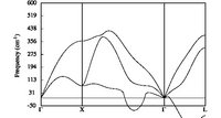
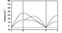
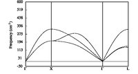
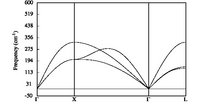
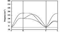
From a long time now, I am trying to get nice phonon dispersion curves for simple metals in the simple FCC structure (primitive cell, rhomboedral structure).

Using the tutorial provided on the abinit website, and using the provided Al pseudopotential (13al.981214.fhi), I can obtain the wanted phonon dispersion curve.

The problem occurs when using LDA PAW atomic data. I just cannot obtain a correct dispersion curves. Whatever I do, it is just no correct. I tried to increase accuracy and it makes no changes. I also tried different Self-Consistent-Field cycles and it makes no difference. With abinit 7.0.3, one can now test the pawxcdev parameter, and again, no more improvements. I though that it could come from the PAW I used, even if tests were ok, so I made test with other elements (Au) and the results are even worst.

Actually, I do not know what to do more. All aids and suggestions are welcome. thanks,

Emile

Typical RF input file:

Code: Select all

# Crystalline Al : computation of the phonon spectrum

   ndtset   9
#Set 1 : ground state self-consistency

  getwfk1   0            # Cancel default
  kptopt1   1            # Automatic generation of k points, taking
                         # into account the symmetry
    nqpt1   0            # Cancel default
  tolvrs1   1.0d-20      # SCF stopping criterion (modify default)
  rfphon1   0            # Cancel default
 
#Q vectors for all datasets

#Complete set of symmetry-inequivalent qpt chosen to be commensurate
# with kpt mesh so that only one set of GS wave functions is needed.
#Generated automatically by running GS calculation with kptopt=1,
# nshift=0, shiftk=0 0 0 (to include gamma) and taking output kpt set
# file as qpt set. Set nstep=1 so only one iteration runs.

     nqpt   1            # One qpt for each dataset (only 0 or 1 allowed)
                         # This is the default for all datasets and must
                         #  be explicitly turned off for dataset 1.

     qpt2   0.00000000E+00  0.00000000E+00  0.00000000E+00
     qpt3   2.50000000E-01  0.00000000E+00  0.00000000E+00
     qpt4   5.00000000E-01  0.00000000E+00  0.00000000E+00
     qpt5   2.50000000E-01  2.50000000E-01  0.00000000E+00
     qpt6   5.00000000E-01  2.50000000E-01  0.00000000E+00
     qpt7  -2.50000000E-01  2.50000000E-01  0.00000000E+00
     qpt8   5.00000000E-01  5.00000000E-01  0.00000000E+00
     qpt9  -2.50000000E-01  5.00000000E-01  2.50000000E-01

#Sets 4-10 : Finite-wave-vector phonon calculations (defaults for all datasets)

   getwfk   1          # Use GS wave functions from dataset1
   kptopt   3          # Need full k-point set for finite-Q response
   rfphon   1          # Do phonon response
  rfatpol   1 1        # Treat displacements of all atoms
    rfdir   1 1 1      # Do all directions (symmetry will be used)
   tolvrs   1.0d-10     # This default is active for sets 3-10

#######################################################################
#Common input variables

#Definition of the unit cell
    acell   3*7.5204497364  # This is equivalent to   10.61 10.61 10.61
    rprim   0.0  0.5  0.5   # In lessons 1 and 2, these primitive vectors 
            0.5  0.0  0.5   # (to be scaled by acell) were 1 0 0  0 1 0  0 0 1 
            0.5  0.5  0.0   # that is, the default.

#Definition of the atom types
   ntypat   1         # There are two types of atom
    znucl   13        # The keyword "znucl" refers to the atomic number of the 
                      # possible type(s) of atom. The pseudopotential(s) 
                      # mentioned in the "files" file must correspond
                      # to the type(s) of atom. Here, type 1 is the Aluminum,
                      # type 2 is the Arsenic.

#Definition of the atoms
    natom   1         # There are two atoms
    typat   1       # The first is of type 1 (Al), the second is of type 2 (As).
                       
     xred   0.0  0.0  0.0

#Gives the number of band, explicitely (do not take the default)
    nband   40         
    occopt   3
    tsmear  300.00 K

#Definition of the planewave basis set

     ecut   40.0           # Maximal kinetic energy cut-off, in Hartree
pawecutdg  120.0
pawxcdev     0

#Definition of the k-point grid
    ngkpt   4  4  4          
  nshiftk   4              # Use one copy of grid only (default)
   shiftk   0.0 0.0 0.5    # This gives the usual fcc Monkhorst-Pack grid
            0.0 0.5 0.0
            0.5 0.0 0.0
            0.5 0.5 0.5

#Definition of the SCF procedure
     iscf   7          # Self-consistent calculation, using algorithm 5
    nstep   2000         # Maximal number of SCF cycles
   diemac   9.0        # Although this is not mandatory, it is worth to
                       # precondition the SCF cycle. The model dielectric
                       # function used as the standard preconditioner
                       # is described in the "dielng" input variable section.
                       # The dielectric constant of AlAs is smaller that the one of Si (=12).
# add to conserve old < 6.7.2 behavior for calculating forces at each SCF step
 optforces 1

typical anaddb input file:

Code: Select all

!Input file for the anaddb code. Analysis of the SiO2 DDB                       

!Flags
 ifcflag   1     ! Interatomic force constant flag

!Wavevector grid number 1 (coarse grid, from DDB)
  brav    2      ! Bravais Lattice : 1-S.C., 2-F.C., 3-B.C., 4-Hex.)
  ngqpt   4  4  4   ! Monkhorst-Pack indices
  nqshft  1         ! number of q-points in repeated basic q-cell
  q1shft  3*0.0

!Effective charges
     asr   1     ! Acoustic Sum Rule. 1 => imposed asymetrically
  chneut   1     ! Charge neutrality requirement for effective charges.

!Interatomic force constant info
  dipdip  1      ! Dipole-dipole interaction treatment

!Phonon band structure output for band2eps - See note near end for
! dealing with gamma LO-TO splitting issue.
   eivec  4

!Wavevector list number 1 (Reduced coordinates and normalization factor)         
  nph1l    81      ! number of phonons in list 1                             
  
  qph1l       0.00000000E+00  0.00000000E+00  0.00000000E+00   1.000  !gamma
              2.50000000E-02  2.50000000E-02  0.00000000E+00   1.000
              5.00000000E-02  5.00000000E-02  0.00000000E+00   1.000
              7.50000000E-02  7.50000000E-02  0.00000000E+00   1.000
              1.00000000E-01  1.00000000E-01  0.00000000E+00   1.000
              1.25000000E-01  1.25000000E-01  0.00000000E+00   1.000
              1.50000000E-01  1.50000000E-01  0.00000000E+00   1.000
              1.75000000E-01  1.75000000E-01  0.00000000E+00   1.000
              2.00000000E-01  2.00000000E-01  0.00000000E+00   1.000
              2.25000000E-01  2.25000000E-01  0.00000000E+00   1.000
              2.50000000E-01  2.50000000E-01  0.00000000E+00   1.000
              2.75000000E-01  2.75000000E-01  0.00000000E+00   1.000
              3.00000000E-01  3.00000000E-01  0.00000000E+00   1.000
              3.25000000E-01  3.25000000E-01  0.00000000E+00   1.000
              3.50000000E-01  3.50000000E-01  0.00000000E+00   1.000
              3.75000000E-01  3.75000000E-01  0.00000000E+00   1.000
              4.00000000E-01  4.00000000E-01  0.00000000E+00   1.000
              4.25000000E-01  4.25000000E-01  0.00000000E+00   1.000
              4.50000000E-01  4.50000000E-01  0.00000000E+00   1.000
              4.75000000E-01  4.75000000E-01  0.00000000E+00   1.000
              5.00000000E-01  5.00000000E-01  0.00000000E+00   1.000 !X
              4.87500000E-01  4.87500000E-01  0.97500000E+00   1.000
              4.75000000E-01  4.75000000E-01  0.95000000E+00   1.000
              4.62500000E-01  4.62500000E-01  0.92500000E+00   1.000
              4.50000000E-01  4.50000000E-01  0.90000000E+00   1.000
              4.37500000E-01  4.37500000E-01  0.87500000E+00   1.000
              4.25000000E-01  4.25000000E-01  0.85000000E+00   1.000
              4.12500000E-01  4.12500000E-01  0.82500000E+00   1.000
              4.00000000E-01  4.00000000E-01  0.80000000E+00   1.000
              3.87500000E-01  3.87500000E-01  0.77500000E+00   1.000
              3.75000000E-01  3.75000000E-01  0.75000000E+00   1.000
              3.62500000E-01  3.62500000E-01  0.72500000E+00   1.000
              3.50000000E-01  3.50000000E-01  0.70000000E+00   1.000
              3.37500000E-01  3.37500000E-01  0.67500000E+00   1.000
              3.25000000E-01  3.25000000E-01  0.65000000E+00   1.000
              3.12500000E-01  3.12500000E-01  0.62500000E+00   1.000
              3.00000000E-01  3.00000000E-01  0.60000000E+00   1.000
              2.87500000E-01  2.87500000E-01  0.57500000E+00   1.000
              2.75000000E-01  2.75000000E-01  0.55000000E+00   1.000
              2.62500000E-01  2.62500000E-01  0.52500000E+00   1.000
              2.50000000E-01  2.50000000E-01  0.50000000E+00   1.000
              2.37500000E-01  2.37500000E-01  0.47500000E+00   1.000
              2.25000000E-01  2.25000000E-01  0.45000000E+00   1.000
              2.12500000E-01  2.12500000E-01  0.42500000E+00   1.000
              2.00000000E-01  2.00000000E-01  0.40000000E+00   1.000
              1.87500000E-01  1.87500000E-01  0.37500000E+00   1.000
              1.75000000E-01  1.75000000E-01  0.35000000E+00   1.000
              1.62500000E-01  1.62500000E-01  0.32500000E+00   1.000
              1.50000000E-01  1.50000000E-01  0.30000000E+00   1.000
              1.37500000E-01  1.37500000E-01  0.27500000E+00   1.000
              1.25000000E-01  1.25000000E-01  0.25000000E+00   1.000
              1.12500000E-01  1.12500000E-01  0.22500000E+00   1.000
              1.00000000E-01  1.00000000E-01  0.20000000E+00   1.000
              8.75000000E-02  8.75000000E-02  0.17500000E+00   1.000
              7.50000000E-02  7.50000000E-02  0.15000000E+00   1.000
              6.25000000E-02  6.25000000E-02  0.12500000E+00   1.000
              5.00000000E-02  5.00000000E-02  0.10000000E+00   1.000
              3.75000000E-02  3.75000000E-02  0.07500000E+00   1.000
              2.50000000E-02  2.50000000E-02  0.05000000E+00   1.000
              1.25000000E-02  1.25000000E-02  0.02500000E+00   1.000
              0.00000000E+00  0.00000000E+00  0.00000000E+00   1.000 !gamma
              2.50000000E-02  2.50000000E-02  2.50000000E-02   1.000
              5.00000000E-02  5.00000000E-02  5.00000000E-02   1.000
              7.50000000E-02  7.50000000E-02  7.50000000E-02   1.000
              1.00000000E-01  1.00000000E-01  1.00000000E-01   1.000
              1.25000000E-01  1.25000000E-01  1.25000000E-01   1.000
              1.50000000E-01  1.50000000E-01  1.50000000E-01   1.000
              1.75000000E-01  1.75000000E-01  1.75000000E-01   1.000
              2.00000000E-01  2.00000000E-01  2.00000000E-01   1.000
              2.25000000E-01  2.25000000E-01  2.25000000E-01   1.000
              2.50000000E-01  2.50000000E-01  2.50000000E-01   1.000
              2.75000000E-01  2.75000000E-01  2.75000000E-01   1.000
              3.00000000E-01  3.00000000E-01  3.00000000E-01   1.000
              3.25000000E-01  3.25000000E-01  3.25000000E-01   1.000
              3.50000000E-01  3.50000000E-01  3.50000000E-01   1.000
              3.75000000E-01  3.75000000E-01  3.75000000E-01   1.000
              4.00000000E-01  4.00000000E-01  4.00000000E-01   1.000
              4.25000000E-01  4.25000000E-01  4.25000000E-01   1.000
              4.50000000E-01  4.50000000E-01  4.50000000E-01   1.000
              4.75000000E-01  4.75000000E-01  4.75000000E-01   1.000
              5.00000000E-01  5.00000000E-01  5.00000000E-01   1.000 !L

!Wavevector list number 2 (Cartesian directions for non-analytic gamma phonons)

!The output for this calculation must be cut-and-pasted into the
! t59_out.freq file to be used as band2eps input to get proper LO-TO
! splitting at gamma.  Note that gamma occurrs twice.

  nph2l    1       ! number of directions in list 2

  qph2l   1.0  0.0  0.0    0.0
# This line added when defaults were changed (v5.3) to keep the previous, old behaviour
  symdynmat 0

blackburn · Post by **blackburn** » Fri Dec 07, 2012 2:13 pm

You should increase your k-grid a lot. For a metal, you want an adequate description of the Fermi surface in your ground state calculation which implies a dense k-grid. Depending on your computational resources, you might want to go up to something around ngkpt 20 20 20 (even more if you can). This means you can improve your q-grid also.

Good luck,
Simon

Emile · Post by **Emile** » Fri Dec 07, 2012 2:55 pm

Dear Simon,

Thank you for your quick answer. Since results look good with the first pseudopotential I though that such k-points grids should be fine.
It is also much more time consuming, thus this is the only point I did not really test yet. Well, I used such dense k-points grid for GS calculation but not for RF.
I will do it, and I will show the corresponding results.
Thanks again,

Emile

Emile · Post by **Emile** » Tue Jan 15, 2013 4:07 pm

Dear abiniters,

I made phonon dispersion curves increasing K-points and Q-points as discussed with Simon.

I got the expected phonon dispersion curve with a K-point grid of 16x16x16 and a Q-point grid of 4x4x4 (figure 1).
When I increased the number of K-points to 20x20x20, I got an almost similar curve (figure 2) which should indicate that the convergence is reached.

Then, in order to test the convergence with respect to the Q-point grid I made a calculation with a K-point grid of 18x18x18 and a Q-point grid of 6x6x6. I expected to get a curve similar to the previous ones, but it is different (see figure 3).

Experimental data is close to figure 1 and 2 (http://prola.aps.org/abstract/PR/v143/i2/p487_1). As a consequence, I do not really understand results of figure 3. Maybe it is related to discontinuities from Q-point grid to other Q-point grid, and I am going to investigate this point, but if someone has a better idea, please, let me know.

Thanks,
Emile

ABINIT Discussion Forums

Improving phonon dispersion curves

Improving phonon dispersion curves

Re: Improving phonon dispersion curves

Re: Improving phonon dispersion curves

Re: Improving phonon dispersion curves