Si_band by Abinit+Wannier90
Si_band by Abinit+Wannier90
Dear all
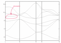
I've studied the steps to calculate a band structure by Abinit+wannier90. I followed the tutorial tw90_4 for Si. The run was OK but the resulting band appears to have a fluctuation along the L-to-G path of the 5th band (the lowest conduction band). Please see the attached band plot. I increased the ecut to 24 to get the reasonably converged ground state density and wave function, and also tried changing around some parameters in the _w90.win file, but still could not get the non-fluctuated line along the mentioned path. The fluctuation even grew bigger when I used sp3 as initial projections. This is rather strange when compared to the Si band obtained from the example provided in the wannier90 package, using the same initial projections. What might be the cause of this result? Am I missing something?. All comments and suggestions are greatly appreciated.
Kind regards,
Thanusit Burinprakhon
PS. I use Abinit 6.4.1 (MPI version, prepared for a x86_64_linux_gnu4.4 computer). The job was run in serial.
The abinit input file is attached. The _w90.win file is exactly the same as that of the tutorial and not attached.
- Attachments
-
 tw90_4.in
- (1.19 KiB) Downloaded 498 times
Re: Si_band by Abinit+Wannier90
Have you made a convergence study in terms of k-points? You can improve your results by increasing the number of k-points given to Wannier90. The Hamiltonian in real space H(R) will be defined on more points and the interpolation on the k-grid will be more accurate.
Simon
Simon
Re: Si_band by Abinit+Wannier90
The above result was obtained with ngkpt 444. I tried ngkpt 888 but it didn't help. In fact, the example given in wannier90 package with ngkpt 444 gives a sensible result. So, I think ngkpt is not the key factor responsible for this strange band shape.
Thanusit
Thanusit
Re: Si_band by Abinit+Wannier90
Deal all
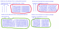
I compared the data in the *.amn and *.mmm files (for Si) obtained from running Abinit tutorial tw90_4 to those provided by example3 in the wannier90 package. The values of data in the same row of the 4th column of the two *.amn file are quite different. Similar behaviour can be observed for those in the 5th column. There are also large differences between the values of data in the *.mmm files from the two sources. Please see the attached image containing the first few lines of each of the files.
Are these suggesting anything?
I checked the list of known problems (in ../doc/abinit/known_problems/known_problems.4.6.x) and found one which seems to involve Wannier function as followed:
P402. (XG021227)
NUMERICAL ERROR
LIKELY GENERAL
Lattice Wannier Function only.
I'm not sure if this problem has been fixed in abinit 6.4.1. If not, could it be the source of the above differences of the calculated data and, hence, lead to the strange Si band structure I got.
Kind regards,
Thanusit
Re: Si_band by Abinit+Wannier90
Your .mmn file would be your problem. Have you tried plotting the band structure with Abinit? If so, do you see the same feature? I believe your problem is from your input file, not from Wannier90. The mmn file is the overlap matrix < u_m (k) | u_n (k+b) >. It will differ from the trial case if you have different wavefunctions (more or less ecut, kpt, etc.).
Can you post your input file please?
Can you post your input file please?
Re: Si_band by Abinit+Wannier90
Thank you for your reply. Please see my input files in the attachments.
Kind regards,
Thanusit
Kind regards,
Thanusit
- Attachments
-
 tw90_4.in
- Abinit input file
- (1.19 KiB) Downloaded 513 times
-
 tw90_4o_DS3_w90.in
- Wannier input file ( its extension is modified to ".in" in stead of ".win " just to make it be allowed for uploading)
- (6.06 KiB) Downloaded 478 times
Re: Si_band by Abinit+Wannier90
You can increase nband in the dataset 1 and use a better k-point grid with non-zero shiftk. This is an FCC system, so
nshiftk 4
shiftk 0.5 0.5 0.5
0.5 0.0 0.0
0.0 0.5 0.0
0.0 0.0 0.5
is good (for the dataset 1 only).
If this doesn't work, you should consider not doing a disentanglement procedure with Wannier90. I found that this can quite mess up your band structure in some case.
nshiftk 4
shiftk 0.5 0.5 0.5
0.5 0.0 0.0
0.0 0.5 0.0
0.0 0.0 0.5
is good (for the dataset 1 only).
If this doesn't work, you should consider not doing a disentanglement procedure with Wannier90. I found that this can quite mess up your band structure in some case.
Re: Si_band by Abinit+Wannier90
Hi,
I tried the k-point grid with non-zero shiftk as listed above but it doesn't work. Disable the disentanglement procedure by setting:
Num_wann = 8,
Num_ band =14,
Exclude_bands = 9-14,
doesn't work either. The fluctuation is not affected by these settings at all.
Kind regards,
Thanusit
I tried the k-point grid with non-zero shiftk as listed above but it doesn't work. Disable the disentanglement procedure by setting:
Num_wann = 8,
Num_ band =14,
Exclude_bands = 9-14,
doesn't work either. The fluctuation is not affected by these settings at all.
Kind regards,
Thanusit
Re: Si_band by Abinit+Wannier90
The non-zero shiftk should be applied only to the density calculation (dataset 1), not the wavefunction (dataset 2).
Otherwise, does increasing the number of Wannier functions in W90 helps?
Otherwise, does increasing the number of Wannier functions in W90 helps?
Re: Si_band by Abinit+Wannier90
Hi
I did used the non-zero shiftk only for the density calculation. It doesn't help.
I'd like to try increasing the number of wannier functions but I'm not sure how to specify the initial projections for the additional WFs. Is there any example of doing this?
Kind regards,
Thanusit
I did used the non-zero shiftk only for the density calculation. It doesn't help.
I'd like to try increasing the number of wannier functions but I'm not sure how to specify the initial projections for the additional WFs. Is there any example of doing this?
Kind regards,
Thanusit
Re: Si_band by Abinit+Wannier90
You can uncomment the bonding orbitals:
!f=0.125,0.125,0.125 : l=0, mr=1 : zona= 0.5
!f=0.625,0.125,0.125 : l=0, mr=1 : zona= 0.5
!f=0.125,0.625,0.125 : l=0, mr=1 : zona= 0.5
!f=0.125,0.125,0.625 : l=0, mr=1 : zona= 0.5
(remove the !) or just add a line:
random
after the "begin projections" line. This will add the required number of projections in the form of s orbitals at a random point. The system might be longer to converge however (if it converges).
Re: Si_band by Abinit+Wannier90
Hi
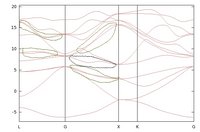
I increased the number of Wannier functions to 12, with the four additional initial projections suggested above. The band seems to get worse. The fluctuation along the L-G path of the 5th band is removed. Please see the attached band plot(Si-band_12WFs.jpg). However, other fluctuations arises along the other paths, for example one along the G-X path (bound by the black closed line). In addition, there appears the splitting of lines along several sections (highlighted by the green closed lines).
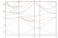
I've tried several combinations of the initial projections. The mixing up between sp3, bonding, and anti-bonding orbitals always gives poor band structure. There is an interesting result in which the suspicious fluctuation is removed but the small line splitting remains in some sections (bound by green closed lines in the attached band plot Si_band_32WFs.jpg). I used 32 WFs and the sp3 orbitals on each of 8 different sites (bond centres) as the initial projections. Is this sensible? If so, is there any other way to further fine tuning this result?
Kind regards,
Thanusit
Re: Si_band by Abinit+Wannier90
Is your total spread well converged?
You can look at this by using:
grep CONV wannier90.wout
The total spread is the 4th column. If the convergence is poor (it happens often), you would need to increase the number of k-points in dataset 2 and 3.
You can look at this by using:
grep CONV wannier90.wout
The total spread is the 4th column. If the convergence is poor (it happens often), you would need to increase the number of k-points in dataset 2 and 3.
Re: Si_band by Abinit+Wannier90
Hi
The result of grep CONV *_w90.wout is as attached. The extracted data for iterations 90-100 are listed below. The spread convergence is not better than 0.1 Ang^2. I think this is poor. How about the RMS Gradient, are they too large?
+-----------------------------------------------------------------------------------------------+<-- CONV
| Iter Delta Spread RMS Gradient Spread (Ang^2) Time |<-- CONV
+----------------------------------------------------------------------------------------------+<-- CONV
.....
90 0.856E+00 0.8992899749 67.0131918763 85.83 <-- CONV
91 -0.252E+00 15.5568687346 66.7607285782 86.67 <-- CONV
92 -0.231E+00 7.6402851083 66.5293140687 87.52 <-- CONV
93 -0.254E+00 2.1791844041 66.2751910830 88.36 <-- CONV
94 -0.182E+00 1.0553204274 66.0928862540 89.20 <-- CONV
95 -0.238E-01 0.9939694940 66.0690416161 90.05 <-- CONV
96 -0.429E-01 0.6107963222 66.0261676939 90.90 <-- CONV
97 -0.252E-01 0.5185084924 66.0009378084 91.75 <-- CONV
98 -0.369E-01 0.5832314047 65.9640148707 92.60 <-- CONV
99 -0.376E-01 1.0786134257 65.9264614153 93.45 <-- CONV
100 -0.152E-01 0.4215962468 65.9112592193 94.30 <-- CONV
Kind regards,
Thanusit
- Attachments
-
 grep_CONV.in
- The output from grep CONV *_w90.wout
- (8.13 KiB) Downloaded 446 times
Re: Si_band by Abinit+Wannier90
This is indeed large. To improve upon this, you could change your initial projections. I recommend using the sp3 on Si and the bonding orbitals. However, you shouldn't use r=4 for the sp3 orbitals as you are using a pseudopotential, not a full atomic wavefunction. r=1 (the default value) should be better.
You can also increase num_iter to 1000 (or more) to improve the convergence.
You can also increase num_iter to 1000 (or more) to improve the convergence.
Re: Si_band by Abinit+Wannier90
Hi
Please note that the total spread given in my previous post is corresponding to the calculation with 32 Wannier functions and sp3 initial projections. With this condition, I tried using num_iter = 1000 and r=1 but the convergence remains poor (not better than 0.1 Ang^2). I guess my initial projections are not right.
I went back to check the total spread obtained from running the input files given earlier, i.e. the original tw90_4 tutorial (with ecut 24) which results in the band fluctuation along the L-G path as shown in my first post. It is very well converged, though, as shown below. Does it mean that the number of Wannier functions and the initial projections used in the tutorial are already good? If so, what else might lead to the strange fluctuation?
+----------------------------------------------------------------------------------------------+<-- CONV
| Iter Delta Spread RMS Gradient Spread (Ang^2) Time |<-- CONV
+----------------------------------------------------------------------------------------------+<-- CONV
......
90 -0.114E-12 0.0000001893 22.5279828245 17.62 <-- CONV
91 0.568E-13 0.0000001858 22.5279828245 17.66 <-- CONV
92 -0.355E-13 0.0000001857 22.5279828245 17.69 <-- CONV
93 -0.355E-13 0.0000001851 22.5279828245 17.71 <-- CONV
94 0.128E-12 0.0000001767 22.5279828245 17.74 <-- CONV
95 -0.320E-13 0.0000001764 22.5279828245 17.76 <-- CONV
96 -0.711E-13 0.0000001748 22.5279828245 17.78 <-- CONV
97 0.497E-13 0.0000001716 22.5279828245 17.81 <-- CONV
98 -0.107E-13 0.0000001711 22.5279828245 17.83 <-- CONV
99 -0.142E-13 0.0000001650 22.5279828245 17.86 <-- CONV
100 -0.568E-13 0.0000001642 22.5279828245 17.88 <-- CONV
Kind regards,
Thanusit
Re: Si_band by Abinit+Wannier90
Hi
I think I've got, at least partially, the solution for the above problem. Above all, many thanks to Dr. D.R. Hamann for his kind suggestions that it is crucial to pay a lot of attention on the disentangle energy windows. This is what I missed in the first place. After experimenting with the energy windows (via input parameters: dis_win_min, dis_win_max, dis_froz_min, and dis_froz_max), I've found that to get a decent interpolated Si band structure (with psp: 14si.pspnc, ecut=12, sp3 initial projection):
1. the k-grid density should be at least 6 6 6, and
2. for a given number of Wannier functions and a numbers of bands entering the interpolation, the disentangle windows must be precisely selected.
However, to find the proper energy windows, the way I did was rather trial and errors. I wonder if there is a common criteria for selecting these energy windows. For this, I've tried to study the related papers suggested in the tutorial but, I have to confess, my theoretical background is simply not enough to get me the answer. Comments and suggestions from experts would greatly help.
Kind regards,
Thanusit


