LDA+U calculations

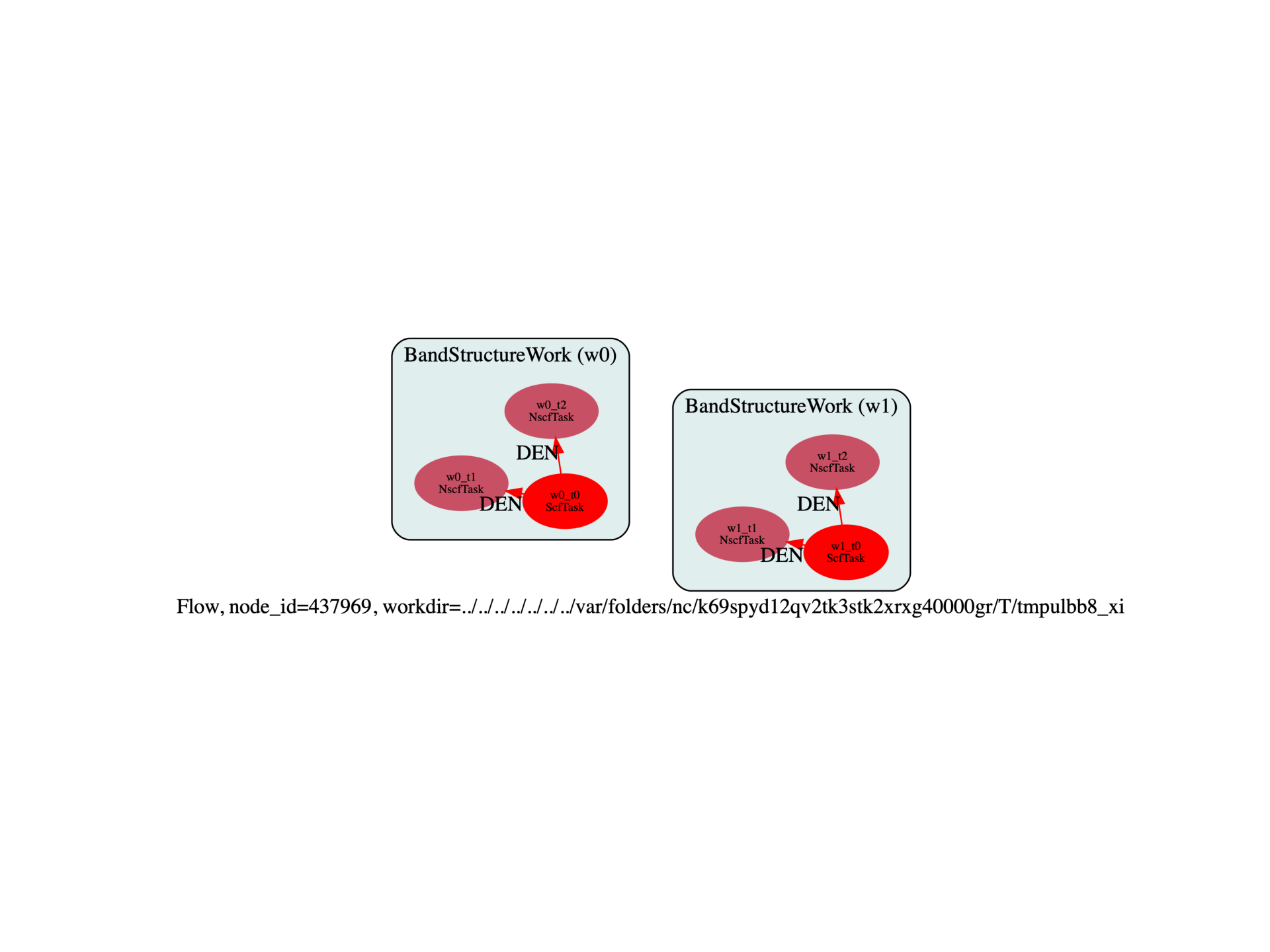
This example shows how to compute the LDA+U band structure of NiO with PAW for several values of U-J.

import sys
import os
import abipy.data as abidata
import abipy.abilab as abilab
import abipy.flowtk as flowtk

from abipy.flowtk.abiobjects import LdauParams


def make_scf_nscf_dos_inputs(structure, pseudos, luj_params, paral_kgb=1):
    # Input file taken from tldau_2.in
    multi = abilab.MultiDataset(structure, pseudos=pseudos, ndtset=3)

    # Global variables
    global_vars = dict(
        #
        ecut=12,
        pawecutdg=30,
        nband=40,
        occopt=7,
        tsmear=0.015,
        nstep=50,
        paral_kgb=paral_kgb,
        #
        # Spin
        nsppol=1,
        nspden=2,
        nspinor=1,
        spinat=[0,  0,  1,
                0,  0, -1,
                0,  0,  0,
                0,  0,  0],
        # Kpoint Grid
        # The k point grid is not symmetric, but the calculations being
        # for the ground-state, this is not a problem.
    )

    multi.set_vars(global_vars)
    multi.set_vars(luj_params.to_abivars())

    # GS run.
    multi[0].set_vars(
        iscf=17,
        toldfe=1.0e-8,
        ngkpt=[2, 2, 2],
        chksymbreak=0,
    )

    # Band structure run.
    multi[1].set_kpath(ndivsm=6)
    multi[1].set_vars(tolwfr=1e-10)

    # DOS calculation.
    multi[2].set_vars(
        iscf=-3,   # NSCF calculation
        ngkpt=structure.calc_ngkpt(nksmall=8),
        shiftk=[0.0, 0.0, 0.0],
        nshiftk=1,
        tolwfr=1.e-8,
        #pawprtdos=1,
    )

    # Generate two input files for the GS and the NSCF run
    scf_input, nscf_input, dos_input = multi.split_datasets()

    return scf_input, nscf_input, dos_input


def build_flow(options):
    # Working directory (default is the name of the script with '.py' removed and "run_" replaced by "flow_")
    if not options.workdir:
        options.workdir = os.path.basename(sys.argv[0]).replace(".py", "").replace("run_", "flow_")

    flow = flowtk.Flow(options.workdir, manager=options.manager)

    # Create the work for the band structure calculation.
    structure = abidata.structure_from_ucell("NiO")
    pseudos = abidata.pseudos("28ni.paw", "8o.2.paw")

    # The code below set up the parameters for the LDA+U calculation in NiO.
    #usepawu   1
    #lpawu   2 -1
    #upawu  8.0 0.0 eV
    #jpawu  0.8 0.0 eV
    usepawu = 1
    u_values = [5.0, 8.0]

    for u in u_values:
        # Apply U-J on Ni only.
        luj_params = LdauParams(usepawu, structure)
        luj_params.luj_for_symbol("Ni", l=2, u=u, j=0.1*u, unit="eV")

        scf_input, nscf_input, dos_input = make_scf_nscf_dos_inputs(structure, pseudos, luj_params)

        work = flowtk.BandStructureWork(scf_input, nscf_input, dos_inputs=dos_input)
        flow.register_work(work)

    return flow


# This block generates the thumbnails in the AbiPy gallery.
# You can safely REMOVE this part if you are using this script for production runs.
if os.getenv("READTHEDOCS", False):
    __name__ = None
    import tempfile
    options = flowtk.build_flow_main_parser().parse_args(["-w", tempfile.mkdtemp()])
    build_flow(options).graphviz_imshow()


@flowtk.flow_main
def main(options):
    """
    This is our main function that will be invoked by the script.
    flow_main is a decorator implementing the command line interface.
    Command line args are stored in `options`.
    """
    return build_flow(options)


if __name__ == "__main__":
    sys.exit(main())

Run the script with:

run_ldaus.py -s

then use:

abirun.py flow_ldaus/ ebands

to analyze all GSR files produced by flow.

KS electronic bands:
       nsppol  nspinor  nspden  nkpt  nband  nelect  fermie formula  natom  \
w0_t0       1        1       2     3     40    48.0   6.084  Ni2 O2      4
w0_t1       1        1       2   129     40    48.0   6.084  Ni2 O2      4
w0_t2       1        1       2   213     40    48.0   6.169  Ni2 O2      4
w1_t0       1        1       2     3     40    48.0   6.855  Ni2 O2      4
w1_t1       1        1       2   129     40    48.0   6.855  Ni2 O2      4
w1_t2       1        1       2   213     40    48.0   6.432  Ni2 O2      4

       angle0  angle1  angle2      a      b      c  volume abispg_num  \
w0_t0    60.0    60.0    60.0  2.964  2.964  5.927  36.809        166
w0_t1    60.0    60.0    60.0  2.964  2.964  5.927  36.809        166
w0_t2    60.0    60.0    60.0  2.964  2.964  5.927  36.809        166
w1_t0    60.0    60.0    60.0  2.964  2.964  5.927  36.809        166
w1_t1    60.0    60.0    60.0  2.964  2.964  5.927  36.809        166
w1_t2    60.0    60.0    60.0  2.964  2.964  5.927  36.809        166

         scheme  occopt  tsmear_ev  bandwidth_spin0  fundgap_spin0  \
w0_t0  gaussian       7      0.408           99.343          3.324
w0_t1  gaussian       7      0.408           99.680          3.049
w0_t2  gaussian       7      0.408           99.838          2.560
w1_t0  gaussian       7      0.408           99.318          4.626
w1_t1  gaussian       7      0.408           99.628          3.352
w1_t2  gaussian       7      0.408           99.826          3.155

       dirgap_spin0 task_class                               ncfile  node_id  \
w0_t0         3.351    ScfTask  flow_ldaus/w0/t0/outdata/out_GSR.nc   241313
w0_t1         3.352   NscfTask  flow_ldaus/w0/t1/outdata/out_GSR.nc   241314
w0_t2         3.041   NscfTask  flow_ldaus/w0/t2/outdata/out_GSR.nc   241315
w1_t0         4.626    ScfTask  flow_ldaus/w1/t0/outdata/out_GSR.nc   241317
w1_t1         3.928   NscfTask  flow_ldaus/w1/t1/outdata/out_GSR.nc   241318
w1_t2         3.983   NscfTask  flow_ldaus/w1/t2/outdata/out_GSR.nc   241319

                   status
w0_t0  Completed
w0_t1  Completed
w0_t2  Completed
w1_t0  Completed
w1_t1  Completed
w1_t2  Completed

The second task in each work (w*_t1) is a NSCF run along the high symmetry path. and we can compare the results of these two task by specifying the node identifiers:

abirun.py flow_ldaus/ ebands -p –nids=241314,241318