wannier90 Package

Contents

• wannier90 Package

  • wannier90 Module

  • abiwan Module

  • win Module

  • wout Module

wannier90 Module

abiwan Module

Interface to the ABIWAN netcdf file produced by abinit when calling wannier90 in library mode. Inspired to the Fortran version of wannier90.

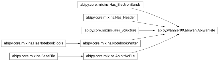
class abipy.wannier90.abiwan.AbiwanFile(filepath)

Bases: abipy.core.mixins.AbinitNcFile, abipy.core.mixins.Has_Header, abipy.core.mixins.Has_Structure, abipy.core.mixins.Has_ElectronBands, abipy.core.mixins.NotebookWriter

File produced by Abinit with the unitary matrices obtained by calling wannier90 in library mode.

Usage example:

with abilab.abiopen("foo_ABIWAN.nc") as abiwan:
    print(abiwan)

Inheritance Diagram

classmethod from_file(filepath)

Initialize the object from a netcdf file.

nwan_spin()

Number of Wannier functions for each spin.

mwan()

Max number of Wannier functions over spins, i.e max(nwan_spin) Used to dimension arrays.

nntot()

Number of k-point neighbours.

bands_in()

[nsppol, mband] logical array. Set to True if (spin, band) is included in the calculation. Set by exclude_bands

lwindow()

[nsppol, nkpt, max_num_bands] array. Only if disentanglement. True if this band at this k-point lies within the outer window

have_disentangled_spin()

[nsppol] bool array. Whether disentanglement has been performed.

wann_centers()

[nsppol, mwan, 3] array with Wannier centers in Ang.

wann_spreads()

[nsppol, mwan] array with spreads in Ang^2

irvec()

[nrpts, 3] array with the lattice vectors in the Wigner-Seitz cell in the basis of the lattice vectors defining the unit cell

ndegen()

[nrpts] array with the degeneracy of each point. It will be weighted using 1 / ndegen[ir]

params()

OrderedDict with parameters that might be subject to convergence studies.

to_string(verbose=0)

String representation with verbosity level verbose.

close()

Close file.

ebands()

abipy.electrons.ebands.ElectronBands object.

property structure

abipy.core.structure.Structure object.

hwan()

Construct the matrix elements of the KS Hamiltonian in real space

interpolate_ebands(vertices_names=None, line_density=20, ngkpt=None, shiftk=(0, 0, 0), kpoints=None)

Build new abipy.electrons.ebands.ElectronBands object by interpolating the KS Hamiltonian with Wannier functions. Supports k-path via (vertices_names, line_density), IBZ mesh defined by ngkpt and shiftk or input list of kpoints.

Parameters

• vertices_names – Used to specify the k-path for the interpolated QP band structure List of tuple, each tuple is of the form (kfrac_coords, kname) where kfrac_coords are the reduced coordinates of the k-point and kname is a string with the name of the k-point. Each point represents a vertex of the k-path. line_density defines the density of the sampling. If None, the k-path is automatically generated according to the point group of the system.

• line_density – Number of points in the smallest segment of the k-path. Used with vertices_names.

• ngkpt – Mesh divisions. Used if bands should be interpolated in the IBZ.

• shiftk – Shifts for k-meshs. Used with ngkpt.

• kpoints – abipy.core.kpoints.KpointList object taken e.g from a previous ElectronBands. Has precedence over vertices_names and line_density.

Returns: abipy.electrons.ebands.ElectronBands object with Wannier-interpolated energies.

get_plotter_from_ebands(ebands)

Interpolate energies using the k-points given in input abipy.electrons.ebands.ElectronBands ebands.

Return: abipy.electrons.ebands.ElectronBandsPlotter object.

yield_figs(**kwargs)

This function generates a predefined list of matplotlib figures with minimal input from the user.

write_notebook(nbpath=None)

Write a jupyter notebook to nbpath. If nbpath is None, a temporay file in the current working directory is created. Return path to the notebook.

class abipy.wannier90.abiwan.HWanR(structure, nwan_spin, spin_vmatrix, spin_rmn, irvec, ndegen)

Bases: abipy.core.skw.ElectronInterpolator

This object represents the KS Hamiltonian in the wannier-gauge representation. It provides low-level methods to interpolate the KS eigenvalues, and a high-level API to interpolate bandstructures and plot the decay of the matrix elements in real space.

# <0n|H|Rm>

eval_sk(spin, kpt, der1=None, der2=None)

Interpolate eigenvalues for all bands at a given (spin, k-point). Optionally compute gradients and Hessian matrices.

Parameters

• spin – Spin index.

• kpt – K-point in reduced coordinates.

• der1 – If not None, ouput gradient is stored in der1[nband, 3].

• der2 – If not None, output Hessian is der2[nband, 3, 3].

Returns

oeigs[nband]

plot(ax=None, fontsize=12, yscale='log', **kwargs)

Plot the matrix elements of the KS Hamiltonian in real space in the Wannier Gauge.

Parameters

• ax – matplotlib.axes.Axes or None if a new figure should be created.

• fontsize – fontsize for legends and titles

• yscale – Define scale for y-axis. Passed to ax.set_yscale

• kwargs – options passed to ax.plot.

Return: matplotlib.figure.Figure

Keyword arguments controlling the display of the figure:

kwargs	Meaning
title	Title of the plot (Default: None).
show	True to show the figure (default: True).
savefig	“abc.png” or “abc.eps” to save the figure to a file.
size_kwargs	Dictionary with options passed to fig.set_size_inches e.g. size_kwargs=dict(w=3, h=4)
tight_layout	True to call fig.tight_layout (default: False)
ax_grid	True (False) to add (remove) grid from all axes in fig. Default: None i.e. fig is left unchanged.
ax_annotate	Add labels to subplots e.g. (a), (b). Default: False
fig_close	Close figure. Default: False.

class abipy.wannier90.abiwan.AbiwanReader(path)

Bases: abipy.electrons.ebands.ElectronsReader

This object reads the results stored in the ABIWAN file produced by ABINIT after having called wannier90 in library mode. It provides helper function to access the most important quantities.

Inheritance Diagram

class abipy.wannier90.abiwan.AbiwanRobot(*args)

Bases: abipy.abio.robots.Robot, abipy.electrons.ebands.RobotWithEbands

This robot analyzes the results contained in multiple ABIWAN.nc files.

Inheritance Diagram

EXT = 'ABIWAN'

get_dataframe(with_geo=True, abspath=False, funcs=None, **kwargs)

Return a pandas.DataFrame with the most important Wannier90 results. and the filenames as index.

Parameters

• with_geo – True if structure info should be added to the dataframe

• abspath – True if paths in index should be absolute. Default: Relative to getcwd().

kwargs:

attrs:

List of additional attributes of the abipy.electrons.gsr.GsrFile to add to the DataFrame.

funcs: Function or list of functions to execute to add more data to the DataFrame.

Each function receives a abipy.electrons.gsr.GsrFile object and returns a tuple (key, value) where key is a string with the name of column and value is the value to be inserted.

plot_hwanr(ax=None, colormap='jet', fontsize=8, **kwargs)

Plot the matrix elements of the KS Hamiltonian in real space in the Wannier Gauge. on the same Axes.

Parameters

• ax – matplotlib.axes.Axes or None if a new figure should be created.

• colormap – matplotlib color map.

• fontsize – fontsize for legends and titles

Return: matplotlib.figure.Figure

Keyword arguments controlling the display of the figure:

kwargs	Meaning
title	Title of the plot (Default: None).
show	True to show the figure (default: True).
savefig	“abc.png” or “abc.eps” to save the figure to a file.
size_kwargs	Dictionary with options passed to fig.set_size_inches e.g. size_kwargs=dict(w=3, h=4)
tight_layout	True to call fig.tight_layout (default: False)
ax_grid	True (False) to add (remove) grid from all axes in fig. Default: None i.e. fig is left unchanged.
ax_annotate	Add labels to subplots e.g. (a), (b). Default: False
fig_close	Close figure. Default: False.

get_interpolated_ebands_plotter(vertices_names=None, knames=None, line_density=20, ngkpt=None, shiftk=(0, 0, 0), kpoints=None, **kwargs)

Parameters

• vertices_names – Used to specify the k-path for the interpolated QP band structure It’s a list of tuple, each tuple is of the form (kfrac_coords, kname) where kfrac_coords are the reduced coordinates of the k-point and kname is a string with the name of the k-point. Each point represents a vertex of the k-path. line_density defines the density of the sampling. If None, the k-path is automatically generated according to the point group of the system.

• knames – List of strings with the k-point labels defining the k-path. It has precedence over vertices_names.

• line_density – Number of points in the smallest segment of the k-path. Used with vertices_names.

• ngkpt – Mesh divisions. Used if bands should be interpolated in the IBZ.

• shiftk – Shifts for k-meshs. Used with ngkpt.

• kpoints – abipy.core.kpoints.KpointList object taken e.g from a previous ElectronBands. Has precedence over vertices_names and line_density.

Return: abipy.electrons.ebands.ElectronBandsPlotter object.

yield_figs(**kwargs)

This function generates a predefined list of matplotlib figures with minimal input from the user. Used in abiview.py to get a quick look at the results.

write_notebook(nbpath=None)

Write a jupyter notebook to nbpath. If nbpath is None, a temporay file in the current working directory is created. Return path to the notebook.

win Module

Interface to the win input file used by Wannier90.

abipy.wannier90.win.structure2wannier90(structure)

Return string with stucture in wannier90 format.

class abipy.wannier90.win.Wannier90Input(structure, comment='', win_args=None, win_kwargs=None, spell_check=True)

Bases: abipy.abio.inputs.AbstractInput, abipy.core.mixins.Has_Structure

This object stores the wannier90 input variables.

Inheritance Diagram

classmethod from_abinit_file(filepath)

Build wannier90 template input file from Abinit input/output file. Possibly with electron bands.

property vars

Dictionary with the input variables. Used to implement the dict-like interface.

set_spell_check(false_or_true)

Activate/Deactivate spell-checking

property spell_check

True if spell checking is activated.

property structure

abipy.core.structure.Structure object.

to_string(sortmode=None, mode='text', verbose=0)

String representation.

Parameters

• sortmode – “a” for alphabetical order, None if no sorting is wanted

• mode – Either text or html if HTML output with links is wanted.

set_kpath(bands_num_points=100, qptbounds=None)

Set the variables for the computation of the electronic band structure.

Parameters

• bands_num_points – The number of points along the first section of the bandstructure plot given by kpoint_path. Other sections will have the same density of k-points

• qptbounds – q-points defining the path in k-space. If None, we use the default high-symmetry k-path defined in the pymatgen database.

wout Module

Interface to the wout output file produced by Wannier90.

class abipy.wannier90.wout.WoutFile(filepath)

Bases: abipy.core.mixins.BaseFile, abipy.core.mixins.Has_Structure, abipy.core.mixins.NotebookWriter

Main output file produced by Wannier90

Usage example:

with abilab.abiopen("foo.wout") as wout:
    print(wout)
    wout.plot()

Inheritance Diagram

close()

Close file. Required by abc protocol.

to_string(verbose=0)

String representation.

property structure

abipy.core.structure.Structure object.

plot(fontsize=12, **kwargs)

Plot the convergence of the Wannierise cycle.

Parameters

fontsize – legend and label fontsize.

Returns: matplotlib.figure.Figure

Keyword arguments controlling the display of the figure:

kwargs	Meaning
title	Title of the plot (Default: None).
show	True to show the figure (default: True).
savefig	“abc.png” or “abc.eps” to save the figure to a file.
size_kwargs	Dictionary with options passed to fig.set_size_inches e.g. size_kwargs=dict(w=3, h=4)
tight_layout	True to call fig.tight_layout (default: False)
ax_grid	True (False) to add (remove) grid from all axes in fig. Default: None i.e. fig is left unchanged.
ax_annotate	Add labels to subplots e.g. (a), (b). Default: False
fig_close	Close figure. Default: False.

plot_centers_spread(fontsize=8, **kwargs)

Plot the convergence of the Wannier centers and spread as function of iteration number

Parameters

fontsize – legend and label fontsize.

Returns: matplotlib.figure.Figure

Keyword arguments controlling the display of the figure:

kwargs	Meaning
title	Title of the plot (Default: None).
show	True to show the figure (default: True).
savefig	“abc.png” or “abc.eps” to save the figure to a file.
size_kwargs	Dictionary with options passed to fig.set_size_inches e.g. size_kwargs=dict(w=3, h=4)
tight_layout	True to call fig.tight_layout (default: False)
ax_grid	True (False) to add (remove) grid from all axes in fig. Default: None i.e. fig is left unchanged.
ax_annotate	Add labels to subplots e.g. (a), (b). Default: False
fig_close	Close figure. Default: False.

yield_figs(**kwargs)

This function generates a predefined list of matplotlib figures with minimal input from the user.

write_notebook(nbpath=None)

Write a jupyter notebook to nbpath. If nbpath is None, a temporay file in the current working directory is created. Return path to the notebook.