AbiPy Gallery
There are a variety of ways to use the AbiPy post-processing tools, and some of them are illustrated in the examples in this directory. These examples represent an excellent starting point if you need to implement a customized script to solve your particular problem. Keep in mind, however, that simple visualization tasks can be easily automated by just issuing in the terminal:
abiopen.py FILE --expose
to generate a predefined list of matplotlib plots. To activate the plotly version (if available) use:
abiopen.py FILE --plotly
Note also that one can generate jupyter-lab notebooks directly from the command line with abiopen.py and the command:
abiopen.py FILE -nb
Add –classic-notebook if you prefer classic jupyter notebooks.
Finally, use one of the options of the abiview.py script to plot the results automatically.
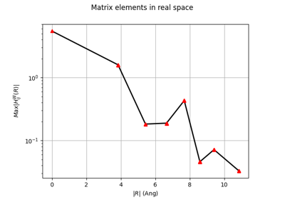
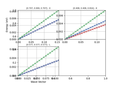
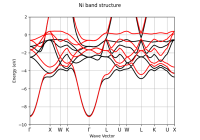
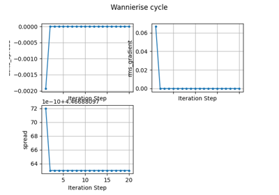
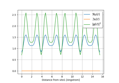
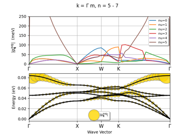
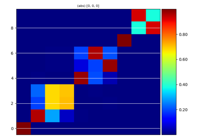
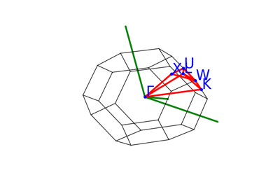
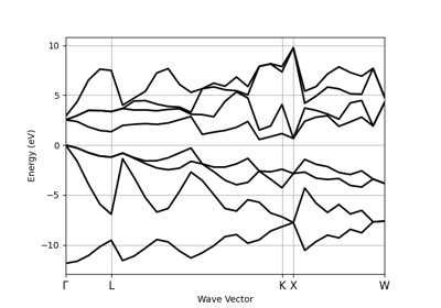
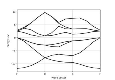
Band structure interpolation with Wannier functions
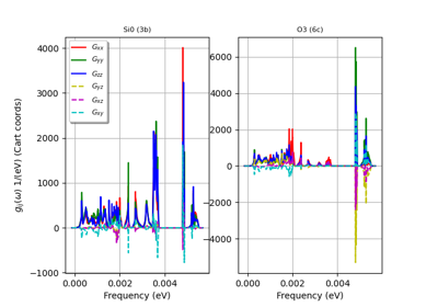
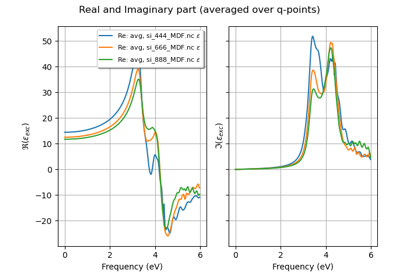
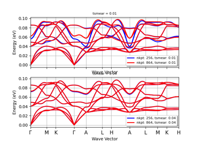

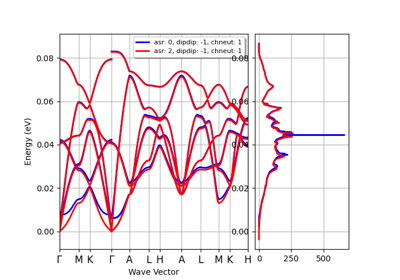
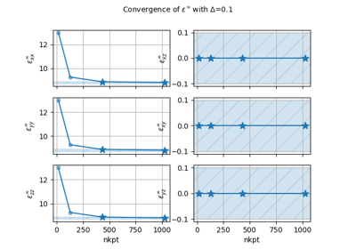
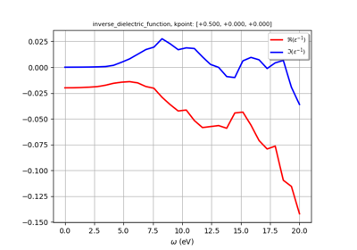
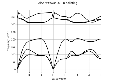
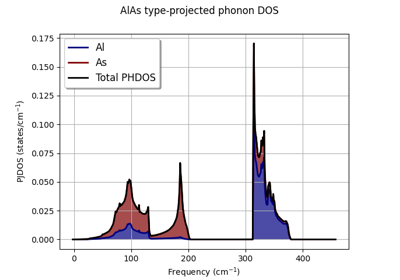
Phonon convergence of ε∞, BECS, phonons and quadrupoles
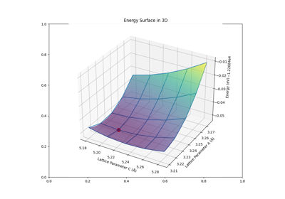

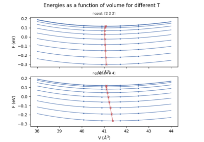
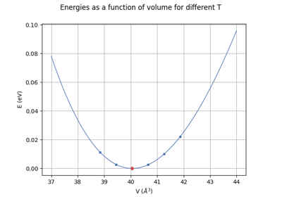
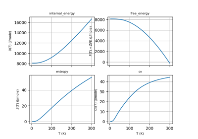
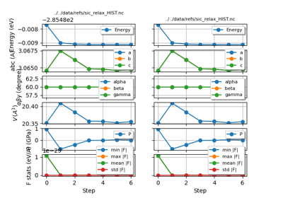
Quasi-harmonic approximation (convergence wrt Q-mesh)