dfpt Package
dpft Package
This subpackage provides objects and functions for the analysis of DFPT calculations.
anaddbnc Module
AnaddbNcFile provides a high-level interface to the data stored in the anaddb.nc file.
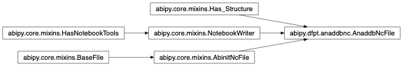
- class abipy.dfpt.anaddbnc.AnaddbNcFile(filepath: str)[source]
Bases:
AbinitNcFile,Has_Structure,NotebookWriterAnaddbNcFile provides a high-level interface to the data stored in the anaddb.nc file. This object is usually instanciated with abiopen(“anaddb.nc”).
- structure[source]
abipy.core.structure.Structureobject.
- ifc[source]
InteratomicForceConstantsobject with the interatomic force constants calculated by anaddb. None, if the netcdf file does not contain the IFCs.
Inheritance Diagram
- classmethod from_file(filepath: str) AnaddbNcFile[source]
Initialize the object from file.
- structure()[source]
Returns the
abipy.core.structure.Structureobject.
- params()[source]
dict with the convergence parameters used to construct
pandas.DataFrame.
- epsinf()[source]
Macroscopic electronic
abipy.tools.tensors.DielectricTensorin Cartesian coordinates (a.k.a. epsilon_infinity) None if the file does not contain this information.
- eps0()[source]
Relaxed ion macroscopic
abipy.tools.tensors.DielectricTensorin Cartesian coordinates (a.k.a. epsilon_zero) None if the file does not contain this information.
- ifc()[source]
The interatomic force constants calculated by anaddb. The following anaddb variables should be used in the run:
ifcflag,natifc,atifc,ifcout. Return None, if the netcdf file does not contain the IFCs,
- dchide()[source]
Non-linear optical susceptibility tensor. Returns a
NLOpticalSusceptibilityTensoror None if the file does not contain this information.
- dchidt()[source]
First-order change in the linear dielectric susceptibility. Returns a list of lists of 3x3 Tensor object with shape (number of atoms, 3). The [i][j] element of the list contains the Tensor representing the change due to the displacement of the ith atom in the jth direction. None if the file does not contain this information.
- oscillator_strength()[source]
A complex
numpy.ndarraycontaining the oscillator strengths with shape [number of phonon modes, 3, 3], in a.u. (1 a.u.=253.2638413 m3/s2). None if the file does not contain this information.
- elastic_data()[source]
Container with the different (piezo)elastic tensors computed by anaddb. stored in pymatgen tensor objects.
- class abipy.dfpt.anaddbnc.AnaddbNcRobot(*args)[source]
Bases:
RobotThis robot analyzes the results contained in multiple anaddb.nc files.
Inheritance Diagram

- EXT = 'anaddb'
- get_elastic_dataframe(with_geo=True, abspath=False, with_params=False, funcs=None, **kwargs) DataFrame[source]
Return a
pandas.DataFramewith properties derived from the elastic tensor and an associated structure. Filename is used as index.- Parameters:
with_geo – True if structure info should be added to the dataframe
abspath – True if paths in index should be absolute. Default: Relative to getcwd().
with_params – False to exclude calculation parameters from the dataframe.
- kwargs:
- attrs:
List of additional attributes of the
abipy.electrons.gsr.GsrFileto add to the DataFrame.- funcs: Function or list of functions to execute to add more data to the DataFrame.
Each function receives a
abipy.electrons.gsr.GsrFileobject and returns a tuple (key, value) where key is a string with the name of column and value is the value to be inserted.
- plot_elastic_properties(fontsize=10, **kwargs)[source]
- Parameters:
fontsize – legend and label fontsize.
Returns:
matplotlib.figure.FigureKeyword arguments controlling the display of the figure:
kwargs
Meaning
title
Title of the plot (Default: None).
show
True to show the figure (default: True).
savefig
“abc.png” or “abc.eps” to save the figure to a file.
size_kwargs
Dictionary with options passed to fig.set_size_inches e.g. size_kwargs=dict(w=3, h=4)
tight_layout
True to call fig.tight_layout (default: False)
ax_grid
True (False) to add (remove) grid from all axes in fig. Default: None i.e. fig is left unchanged.
ax_annotate
Add labels to subplots e.g. (a), (b). Default: False
fig_close
Close figure. Default: False.
plotly
Try to convert mpl figure to plotly.
converters Module
Converters between abinit/abipy format and other external tools. Some portions of the code have been imported from the ConvertDDB.py script developed by Hu Xe, Eric Bousquet and Aldo Romero.
- abipy.dfpt.converters.abinit_to_phonopy(anaddbnc, supercell_matrix, symmetrize_tensors=False, output_dir_path=None, prefix_outfiles='', symprec=1e-05, set_masses=False)[source]
Converts the interatomic force constants(IFC), born effective charges(BEC) and dielectric tensor obtained from anaddb to the phonopy format. Optionally writes the standard phonopy files to a selected directory: FORCE_CONSTANTS, BORN (if BECs are available) POSCAR of the unit cell, POSCAR of the supercell.
The conversion is performed taking the IFC in the Wigner–Seitz supercell with weights as produced by anaddb and reorganizes them in a standard supercell multiple of the unit cell. Operations are vectorized using numpy. This may lead to the allocation of large arrays in case of very large supercells.
Performs a check to verify if the two codes identify the same symmetries and it gives a warning in case of failure. Mismatching symmetries may lead to incorrect conversions.
- Parameters:
anaddbnc – an instance of AnaddbNcFile. Should contain the output of the IFC analysis, the BEC and the dielectric tensor.
supercell_matrix – the supercell matrix used for phonopy. Any choice is acceptable, however the best agreement between the abinit and phonopy results is obtained if this is set to a diagonal matrix with on the diagonal the ngqpt used to generate the anaddb.nc.
symmetrize_tensors – if True the tensors will be symmetrized in the Phonopy object and in the output files. This will apply to IFC, BEC and dielectric tensor.
output_dir_path – a path to a directory where the phonopy files will be created
prefix_outfiles – a string that will be added as a prefix to the name of the written files
symprec – distance tolerance in Cartesian coordinates to find crystal symmetry in phonopy. It might be that the value should be tuned so that it leads to the the same symmetries as in the abinit calculation.
set_masses – if True the atomic masses used by abinit will be added to the PhonopyAtoms and will be present in the returned Phonopy object. This should improve compatibility among abinit and phonopy results if frequencies needs to be calculated.
- Returns:
An instance of a Phonopy object that contains the IFC, BEC and dieletric tensor data.
- abipy.dfpt.converters.phonopy_to_abinit(unit_cell=None, supercell_matrix=None, out_ddb_path=None, ngqpt=None, qpt_list=None, force_constants=None, force_sets=None, phonopy_yaml=None, born=None, primitive_matrix='auto', symprec=1e-05, tolsym=None, nsym=None, supercell=None, calculator=None, manager=None, workdir=None, pseudos=None, verbose=False)[source]
Converts the data from phonopy to an abinit DDB file. The data can be provided in form of arrays or paths to the phonopy files that should be parsed. The minimal input should contains the FORCE_CONSTANTS or FORCE_SETS, or the phonopy.yaml ouput from the postprocessing of phonopy (https://phonopy.github.io/phonopy/output-files.html#phonopy-yaml-and-phonopy-disp-yaml). If BORN is present the Born effective charges (BEC) and dielectric tensor will also be added to the DDB.
The best agreement is obtained with supercell_matrix and ngqpt being equivalent (i.e. supercell_matrix a diagonal matrix with ngqpt as diagonal elements). Non diagonal supercell_matrix are allowed as well, but the information encoded in the DDB will be the result of an interpolation done through phonopy.
Phonopy is used to convert the IFC to the dynamical matrix. However, in order to determine the list of q-points in the irreducible Brillouin zone and to prepare the base for the final DDB file, abinit will be called for a very short and inexpensive run.
Performs a check to verify if the two codes identify the same symmetries and it gives a warning in case of failure. Mismatching symmetries may lead to incorrect conversions.
- Parameters:
unit_cell – a
abipy.core.structure.Structureobject that identifies the unit cell used for the phonopy calculation.supercell_matrix – a 3x3 array representing the supercell matrix used to generated the forces with phonopy.
out_ddb_path – a full path to the file where the new DDB will be written
ngqpt – a list of 3 elements indicating the grid of q points that will be used in the DDB.
qpt_list – alternatively to ngqpt an explicit list of q-points can be provided here. At least one among ngqpt and qpt_list should be defined.
force_constants – an array with shape (num atoms unit cell, num atoms supercell, 3, 3) containing the force constants. Alternatively a string with the path to the FORCE_CONSTANTS file. This or force_sets or phonopy_yaml should be defined. If both given this has precedence.
force_sets – a dictionary obtained from the force sets generated with phonopy. Alternatively a string with the path to the FORCE_SETS file. This or force_constants or phonopy_yaml should be defined.
phonopy_yaml – a filename from the post-processing of phonopy (phonopy.yaml), see https://phonopy.github.io/phonopy/output-files.html#phonopy-yaml-and-phonopy-disp-yaml This or force_constants or force_sets should be dependent. Note that the unit_cel, supercell_matrix, primitive_matrix are included in this file so they do not need to be given.
born – a dictionary with “dielectric” and “born” keywords as obtained from the nac_params in phonopy. Alternatively a string with the path to the BORN file. Notice that the “factor” attribute is not taken into account, so the values should be in default phonopy units.
primitive_matrix – a 3x3 array with the primitive matrix passed to Phonopy. “auto” will use spglib to try to determine it automatically. If the DDB file should contain the actual unit cell this should be the identity matrix.
symprec – distance tolerance in Cartesian coordinates to find crystal symmetry in phonopy. It might be that the value should be tuned so that it leads to the the same symmetries as in the abinit calculation.
tolsym – Gives the tolerance to identify symmetries in abinit. See abinit documentation for more details.
supercell – if given it should represent the supercell used to get the force constants, without any perturbation. It will be used to match it to the phonopy supercell and sort the IFC in the correct order.
calculator – a string with the name of the calculator. Will be used to set the conversion factor for the force constants coming from phonopy.
manager –
abipy.flowtk.tasks.TaskManagerobject. If None, the object is initialized from the configuration filepseudos – List of filenames or list of
pymatgen.io.abinit.pseudos.Pseudoobjects orpymatgen.io.abinit.pseudos.PseudoTableobject. It will be used by abinit to generate the base DDB file. If None the abipy.data.hgh_pseudos.HGH_TABLE table will be used.verbose – verbosity level. Set it to a value > 0 to get more information
workdir – path to the directory where the abinit calculation will be executed.
- Returns:
a DdbFile instance of the file written in out_ddb_path.
- abipy.dfpt.converters.generate_born_deriv(born: dict, zion: Sequence[float] | ndarray, structure: Structure) ndarray[source]
Helper function to generate the portion of the derivatives in the DDB that are related to the Born effective charges and dielectric tensor, starting from the data available in phonopy format.
- Parameters:
born – a dictionary with “dielectric” and “born” keywords as obtained from the nac_params in phonopy.
zion – the ionic charge of each atom in the system. It should be in the same order as the one present in the header of the DDB.
structure – a pymatgen
abipy.core.structure.Structureof the unit cell.
- Returns:
a complex numpy array with shape (len(structure)+2, 3, len(structure)+2, 3). Only the parts relative to the BECs and dielectric tensors will be filled.
- abipy.dfpt.converters.get_dm(phonon, qpt_list: list, structure: Structure) list[source]
Helper function to generate the dynamical matrix in the abinit conventions for a list of q-points from a Phonopy object.
- Parameters:
phonon – a Phonopy object with force constants.
qpt_list – a list of fractional coordinates of q-points for which the dynamical matrix should be generated.
structure – a pymatgen
abipy.core.structure.Structureof the primitive cell.
- Returns:
a list of arrays with the dynamical matrices of the selected q-points.
- abipy.dfpt.converters.add_data_ddb(ddb: DdbFile, dm_list: list, qpt_list: list, born_data) None[source]
Helper function to add the blocks for the dynamical matrix and BECs to a DdbFile object.
- Parameters:
ddb – a DdbFile object to be modified.
dm_list – the list of dynamical matrices to be added.
qpt_list – the list of q-points corresponding to dm_list.
born_data – the data corresponding to BECs and dielectric tensor. If None these part will not be set in the DDB.
- abipy.dfpt.converters.tdep_to_abinit(unit_cell, fc_path, supercell_matrix, supercell, out_ddb_path, ngqpt=None, qpt_list=None, primitive_matrix='auto', lotosplitting_path=None, symprec=1e-05, tolsym=None, manager=None, workdir=None, pseudos=None, verbose=False)[source]
Converts the files produced by TDEP to an abinit DDB file. If the lotosplitting file is provided the BEC and dielectric tensor will also be added to the DDB.
The conversion is performed by first extracting the force constants in phonopy format and then using phonopy_to_abinit_py to generate the DDB file. See the phonopy_to_abinit_py docstring for further details about the second step of the conversion. Notice that the supercell used by TDEP should be provided in order to properly sort the IFC to match the order required by phonopy.
- Parameters:
unit_cell – a
abipy.core.structure.Structureobject that identifies the unit cell used for the TDEP calculation.fc_path – the path to the forceconstants file produced by TDEP.
supercell_matrix – a 3x3 array representing the supercell matrix used to generated the forces with TDEP.
supercell – the supercell used by TDEP to get the force constants, without any perturbation (usually named with extension ssposcar). It will be used to match it to the phonopy supercell and sort the IFC in the correct order.
out_ddb_path – a full path to the file where the new DDB will be written
ngqpt – a list of 3 elements indicating the grid of q points that will be used in the DDB.
qpt_list – alternatively to ngqpt an explicit list of q-points can be provided here. At least one among ngqpt and qpt_list should be defined.
primitive_matrix – a 3x3 array with the primitive matrix passed to Phonopy. “auto” will use spglib to try to determine it automatically. If the DDB file should contain the actual unit cell this should be the identity matrix.
lotosplitting_path – path to the lotosplitting file produced by TDEP. If None no BEC contribution will be set to the DDB.
symprec – distance tolerance in Cartesian coordinates to find crystal symmetry in phonopy. It might be that the value should be tuned so that it leads to the the same symmetries as in the abinit calculation.
tolsym – Gives the tolerance to identify symmetries in abinit. See abinit documentation for more details.
manager –
abipy.flowtk.tasks.TaskManagerobject. If None, the object is initialized from the configuration filepseudos – List of filenames or list of
pymatgen.io.abinit.pseudos.Pseudoobjects orpymatgen.io.abinit.pseudos.PseudoTableobject. It will be used by abinit to generate the base DDB file. If None the abipy.data.hgh_pseudos.HGH_TABLE table will be used.verbose – verbosity level. Set it to a value > 0 to get more information
workdir – path to the directory where the abinit calculation will be executed.
- Returns:
a DdbFile instance of the file written in out_ddb_path.
- abipy.dfpt.converters.parse_tdep_fc(fc_path: str, unit_cell: Structure, supercell) ndarray[source]
Parses a forceconstants file produced by TDEP an converts it to an array in the phonopy format.
- Parameters:
fc_path – path to the forceconstants file
unit_cell – a
abipy.core.structure.Structureobject with the unit cell used for the calculation in TDEP.supercell – the supercell used for the calculation in TDEP.
- Returns:
a comple numpy array with shape (len(unit_cell), len(supercell), 3, 3)
- abipy.dfpt.converters.parse_tdep_lotosplitting(filepath: str) tuple[source]
Parses the lotosplitting file produced by TDEP and transforms them in the phonopy format for Born effective charges and dielectric tensor.
- Parameters:
filepath – path to the lotosplitting file.
- Returns:
a tuple with dielectric tensor and Born effective charges.
- abipy.dfpt.converters.write_tdep_lotosplitting(eps, born, filepath='infile.lotosplitting', fmt='%14.10f') None[source]
Writes an lotosplitting file starting from arrays containing dielectric tensor and Born effective charges.
- Parameters:
eps – a 3x3 array with the dielectric tensor.
born – an array with the Born effective charges.
filepath – the path where the lotosplitting file should be written.
fmt – the format for the float numbers.
- abipy.dfpt.converters.born_to_lotosplitting(born, lotosplitting_path='infile.lotosplitting') None[source]
Converted of a file from the BORN file produced from phonopy to the lotosplitting file used by TDEP.
- Parameters:
born – a dictionary with “dielectric” and “born” keywords as obtained from the nac_params in phonopy. Notice that the “factor” attribute is not taken into account, so the values should be in default phonopy units.
lotosplitting_path – the path where the lotosplitting file should be written.
- abipy.dfpt.converters.write_BORN(primitive, borns, epsilon, filename='BORN', symmetrize_tensors=False) None[source]
Helper function imported from phonopy.file_IO. Contrarily to the original, it does not symmetrize the tensor.
- abipy.dfpt.converters.get_BORN_lines(unitcell, borns, epsilon, factor=None, primitive_matrix=None, supercell_matrix=None, symprec=1e-05, symmetrize_tensors=False) list[source]
Helper function imported from phonopy.file_IO that exposes the option of not symmetrizing the tensor.
- abipy.dfpt.converters.ddb_ucell_to_ddb_supercell(unit_ddb=None, unit_ddb_filepath=None, supercell_ddb_path='out_DDB', nac=True) DdbFile[source]
Convert a DDB file or DDB instance of a unit cell on a q-mesh to the corresponding supercell at q=Gamma.
- Parameters:
unit_ddb – an instance of DDB file.
unit_ddb_filepath – alternatively, a path to the input DDB.
supercell_ddb_path – DDB path of the output DDB on a supercell at Gamma
nac – Set the non-analytical correction
- Returns:
a DdbFile instance and the corresponding DDB file in supercell_ddb_path.
- abipy.dfpt.converters.ddb_ucell_to_phonopy_supercell(unit_ddb=None, unit_ddb_filepath=None, nac=True) Phonopy[source]
Convert a DDB file or DDB instance of a unit cell on a q-mesh to the corresponding supercell at q=Gamma.
- Parameters:
ddb_unit_cell – an instance of DDB file.
unit_ddb_filepath – alternatively, a path to the input DDB.
supercell_ddb_path – DDB path of the output DDB on a supercell at Gamma
nac – Set the non-analytical correction
- Returns:
a Phonopy instance.
ddb Module
Python API for the DDB file containing the derivatives of the total Energy wrt different perturbations.
- exception abipy.dfpt.ddb.AnaddbError(*args, **kwargs)[source]
Bases:
DdbErrorExceptions raised when we try to execute
abipy.flowtk.tasks.AnaddbTaskin theabipy.dfpt.ddb.DdbFilemethodsAn AnaddbError has a reference to the task and to the
EventsReportthat contains the error messages of the run.
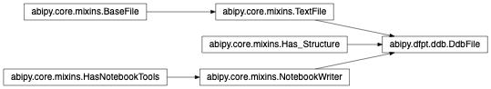
- class abipy.dfpt.ddb.DdbFile(filepath: str)[source]
Bases:
TextFile,Has_Structure,NotebookWriterThis object provides an interface to the DDB file produced by ABINIT as well as methods to compute phonon band structures, phonon DOS, thermodynamic properties etc.
About the indices (idir, ipert) used by Abinit (Fortran notation):
idir in [1, 2, 3] gives the direction (usually reduced direction, cart for strain)
ipert in [1, 2, …, mpert] where mpert = natom + 6
ipert in [1, …, natom] corresponds to atomic perturbations (reduced directions)
ipert = natom + 1 corresponds d/dk (reduced directions)
ipert = natom + 2 corresponds the electric field
ipert = natom + 3 corresponds the uniaxial stress (Cartesian directions)
ipert = natom + 4 corresponds the shear stress. (Cartesian directions)
Inheritance
- exception AnaddbError(*args, **kwargs)
Bases:
DdbErrorExceptions raised when we try to execute
abipy.flowtk.tasks.AnaddbTaskin theabipy.dfpt.ddb.DdbFilemethodsAn AnaddbError has a reference to the task and to the
EventsReportthat contains the error messages of the run.
- classmethod from_string(string: str) DdbFile[source]
Build object from string using temporary file.
- classmethod from_mpid(material_id) DdbFile[source]
Fetch DDB file corresponding to a materials project
material_id, save it to temporary file and return new DdbFile object.Raises: MPRestError if DDB file is not available
- Parameters:
material_id (str) – Materials Project material_id (e.g., mp-1234).
- classmethod as_ddb(obj: Any) DdbFile[source]
Return an instance of
abipy.dfpt.ddb.DdbFilefrom a generic object obj. Accepts: DdbFile or filepath
- property structure: Structure
abipy.core.structure.Structureobject.
- property header
Dictionary with the values reported in the header section. Use e.g.
ddb.header.ecutto access its values
- computed_dynmat()[source]
dict mapping q-point object to –> pandas Dataframe. The
pandas.DataFramecontains the columns: “idir1”, “ipert1”, “idir2”, “ipert2”, “cvalue” and (idir1, ipert1, idir2, ipert2) as index.Note
The indices follow the Abinit (Fortran) notation so they start at 1.
- blocks()[source]
DDB blocks. List of dictionaries, Each dictionary contains the following keys. “qpt” with the reduced coordinates of the q-point. “data” that is a list of strings with the entries of the dynamical matrix for this q-point.
- property qpoints: KpointList
abipy.core.kpoints.KpointListobject with the list of q-points in reduced coordinates.
- qindex(qpoint) int[source]
The index of the q-point in the internal list of q-points. Accepts:
abipy.core.kpoints.Kpointinstance or integer.
- guessed_ngqpt()[source]
Guess for the q-mesh divisions (ngqpt) inferred from the list of q-points found in the DDB file.
Warning
The mesh may not be correct if the DDB file contains points belonging to different meshes and/or the Q-mesh is shifted.
- cart_forces()[source]
Cartesian forces in eV / Ang None if not available i.e. if the GS DDB has not been merged.
- cart_stress_tensor()[source]
abipy.tools.tensors.Stresstensor in cartesian coordinates (GPa units). None if not available.
- has_lo_to_data(select: str = 'at_least_one') bool[source]
True if the DDB file contains the data required to compute the LO-TO splitting.
- has_at_least_one_atomic_perturbation(qpt=None) bool[source]
True if the DDB file contains info on (at least one) atomic perturbation. If the coordinates of a q point are provided only the specified qpt will be considered.
- has_epsinf_terms(select='at_least_one') bool[source]
True if the DDB file contains info on the electric-field perturbation.
- Parameters:
select – Possible values in [“at_least_one”, “at_least_one_diagoterm”, “all”] If select == “at_least_one”, we check if there’s at least one entry associated to the electric field and we assume that anaddb will be able to reconstruct the full tensor by symmetry. “at_least_one_diagoterm” is similar but it only checks for the presence of one diagonal term. If select == “all”, all tensor components must be present in the DDB file.
- has_bec_terms(select: str = 'at_least_one') bool[source]
True if the DDB file contains info on the Born effective charges.
- Parameters:
select – Possible values in [“at_least_one”, “all”] By default, we check if there’s at least one entry associated to atomic displacement and electric field and we assume that anaddb will be able to reconstruct the full tensor by symmetry. If select == “all”, all bec components must be present in the DDB file.
- has_strain_terms(select: str = 'all') bool[source]
True if the DDB file contains info on the (clamped-ion) strain perturbation (i.e. 2nd order derivatives wrt strain)
- Parameters:
select – Possible values in [“at_least_one”, “all”] If select == “at_least_one”, we check if there’s at least one entry associated to the strain. and we assume that anaddb will be able to reconstruct the full tensor by symmetry. If select == “all”, all tensor components must be present in the DDB file.
Note
As anaddb is not yet able to reconstruct the strain terms by symmetry, the default value for select is “all”
- has_internalstrain_terms(select: str = 'all') bool[source]
True if the DDB file contains internal strain terms i.e “off-diagonal” 2nd order derivatives wrt (strain, atomic displacement)
- Parameters:
select – Possible values in [“at_least_one”, “all”] If select == “at_least_one”, we check if there’s at least one entry associated to the strain. and we assume that anaddb will be able to reconstruct the full tensor by symmetry. If select == “all”, all tensor components must be present in the DDB file.
Note
As anaddb is not yet able to reconstruct the strain terms by symmetry, the default value for select is “all”
- has_piezoelectric_terms(select: str = 'all') bool[source]
True if the DDB file contains piezoelectric terms i.e “off-diagonal” 2nd order derivatives wrt (electric_field, strain)
- Parameters:
select – Possible values in [“at_least_one”, “all”] If select == “at_least_one”, we check if there’s at least one entry associated to the strain. and we assume that anaddb will be able to reconstruct the full tensor by symmetry. If select == “all”, all tensor components must be present in the DDB file.
Note
As anaddb is not yet able to reconstruct the (strain, electric) terms by symmetry, the default value for select is “all”
- get_quadrupole_raw_dataframe(with_index_list: bool = False)[source]
Return pandas Dataframe with the dynamical quadrupoles. In with_index_list is True, the list of with the 3 (idir, ipert) tuples is returned. Return None or (None, None) is the DDB does not contain Q*.
Note
These are the raw terms computed with DFPT before the extra symmetrization performed in anaddb.
- has_quadrupole_terms(select: str = 'all') bool[source]
True if the DDB file contains dynamical quadrupoles i.e the 3rd order derivatives wrt (electric_field, atomic_perturbation_gamma, q-wavevector)
- Parameters:
select – Possible values in [“at_least_one”, “all”] If select == “at_least_one”, we check if there’s at least one entry associated to Q* If select == “all”, all tensor components must be present in the DDB file.
Note
As anaddb is not yet able to reconstruct all the Q* entries by symmetry, the default value for select is “all”
- view_phononwebsite(browser=None, verbose=0, dryrun=False, **kwargs)[source]
Invoke anaddb to compute phonon bands. Produce JSON file that can be parsed from the phononwebsite and open it in
browser.- Parameters:
browser – Open webpage in
browser. Use default $BROWSER if None.verbose – Verbosity level
dryrun – Activate dryrun mode for unit testing purposes.
kwargs – Passed to
anaget_phbst_and_phdos_files.
Return: Exit status
- yield_figs(**kwargs)[source]
This function generates a predefined list of matplotlib figures with minimal input from the user.
- yield_plotly_figs(**kwargs)[source]
This function generates a predefined list of plotly figures with minimal input from the user.
- anaget_phmodes_at_qpoint(qpoint=None, asr=2, chneut=1, dipdip=1, dipquad=1, quadquad=1, ifcflag=0, workdir=None, mpi_procs=1, manager=None, verbose=0, lo_to_splitting=False, spell_check=True, directions=None, anaddb_kwargs=None, return_input=False)[source]
Execute anaddb to compute phonon modes at the given q-point. Non analytical contribution can be added if qpoint is Gamma and required elements are present in the DDB.
- Parameters:
qpoint – Reduced coordinates of the qpoint where phonon modes are computed.
asr – Anaddb input variable. See official documentation.
chneut – Anaddb input variable. See official documentation.
dipdip – Anaddb input variable. See official documentation.
dipquad – Anaddb input variable. See official documentation.
quadquad – Anaddb input variable. See official documentation.
workdir – Working directory. If None, a temporary directory is created.
mpi_procs – Number of MPI processes to use.
manager –
abipy.flowtk.tasks.TaskManagerobject. If None, the object is initialized from the configuration fileverbose – verbosity level. Set it to a value > 0 to get more information.
lo_to_splitting – Allowed values are [True, False, “automatic”]. Defaults to False If True the LO-TO splitting will be calculated if qpoint == Gamma and the non_anal_directions non_anal_phfreqs attributes will be addeded to the phonon band structure. “automatic” activates LO-TO if the DDB file contains the dielectric tensor and Born effective charges.
directions – list of 3D directions along which the LO-TO splitting will be calculated. If None the three cartesian direction will be used.
anaddb_kwargs – additional kwargs for anaddb.
return_input – True if
abipy.abio.inputs.AnaddbInputobject should be returned as 2nd argument
Return:
abipy.dfpt.phonons.PhononBandsobject.
- anaget_phmodes_at_qpoints(qpoints=None, asr=2, chneut=1, dipdip=1, dipquad=1, quadquad=1, ifcflag=0, ngqpt=None, workdir=None, mpi_procs=1, manager=None, verbose=0, lo_to_splitting=False, spell_check=True, directions=None, anaddb_kwargs=None, return_input=False)[source]
Execute anaddb to compute phonon modes at the given list of q-points. Non analytical contribution can be added if Gamma belongs to the list and required elements are present in the DDB. If the list of q-points contains points that are not present in the DDB the values will be interpolated provided ifcflag is set to 1.
- Parameters:
qpoints – Reduced coordinates of a list of qpoints where phonon modes are computed.
asr – Anaddb input variable. See official documentation.
chneut – Anaddb input variable. See official documentation.
dipdip – Anaddb input variable. See official documentation.
dipquad – Anaddb input variable. See official documentation.
quadquad – Anaddb input variable. See official documentation.
ifcflag – Anaddb input variable. See official documentation.
ngqpt – Number of divisions for the q-mesh in the DDB file. Auto-detected if None (default).
workdir – Working directory. If None, a temporary directory is created.
mpi_procs – Number of MPI processes to use.
manager –
abipy.flowtk.tasks.TaskManagerobject. If None, the object is initialized from the configuration fileverbose – verbosity level. Set it to a value > 0 to get more information.
lo_to_splitting – Allowed values are [True, False, “automatic”]. Defaults to False If True the LO-TO splitting will be calculated if qpoint == Gamma and the non_anal_directions non_anal_phfreqs attributes will be addeded to the phonon band structure. “automatic” activates LO-TO if the DDB file contains the dielectric tensor and Born effective charges.
directions – list of 3D directions along which the LO-TO splitting will be calculated. If None the three cartesian direction will be used.
anaddb_kwargs – additional kwargs for anaddb.
return_input – True if
abipy.abio.inputs.AnaddbInputobject should be returned as 2nd argument
Return:
abipy.dfpt.phonons.PhononBandsobject.
- anaget_phbst_and_phdos_files(nqsmall=10, qppa=None, ndivsm=20, line_density=None, asr=2, chneut=1, dipdip=1, dipquad=1, quadquad=1, dos_method='tetra', lo_to_splitting='automatic', ngqpt=None, qptbounds=None, anaddb_kwargs=None, with_phonopy_obj=False, verbose=0, spell_check=True, mpi_procs=1, workdir=None, manager=None, return_input=False)[source]
Execute anaddb to compute the phonon band structure and the phonon DOS. Return contex manager that closes the files automatically.
Important
Use:
- with ddb.anaget_phbst_and_phdos_files(…) as g:
phbst_file, phdos_file = g[0], g[1]
to ensure the netcdf files are closed instead of:
phbst_file, phdos_file = ddb.anaget_phbst_and_phdos_files(…)
- Parameters:
nqsmall – Defines the homogeneous q-mesh used for the DOS. Gives the number of divisions used to sample the smallest lattice vector. If 0, DOS is not computed and (phbst, None) is returned.
qppa – Defines the homogeneous q-mesh used for the DOS in units of q-points per reciprocal atom. Overrides nqsmall.
ndivsm – Number of division used for the smallest segment of the q-path.
line_density – Defines the a density of k-points per reciprocal atom to plot the phonon dispersion. Overrides ndivsm.
asr – Anaddb input variable. See official documentation.
chneut – Anaddb input variable. See official documentation.
dipdip – Anaddb input variable. See official documentation.
dipquad – Anaddb input variable. See official documentation.
quadquad – Anaddb input variable. See official documentation.
dos_method – Technique for DOS computation in Possible choices: “tetra”, “gaussian” or “gaussian:0.001 eV”. In the later case, the value 0.001 eV is used as gaussian broadening.
lo_to_splitting – Allowed values are [True, False, “automatic”]. Defaults to “automatic” If True the LO-TO splitting will be calculated and the non_anal_directions and the non_anal_phfreqs attributes will be addeded to the phonon band structure. “automatic” activates LO-TO if the DDB file contains the dielectric tensor and Born effective charges.
ngqpt – Number of divisions for the q-mesh in the DDB file. Auto-detected if None (default).
qptbounds – Boundaries of the path. If None, the path is generated from an internal database depending on the input structure.
anaddb_kwargs – additional kwargs for anaddb.
with_phonopy_obj – if True the IFC will be calculated and used to generate an instance of a Phonopy object as an attribute of PhononBands.
verbose – verbosity level. Set it to a value > 0 to get more information.
mpi_procs – Number of MPI processes to use.
workdir – Working directory. If None, a temporary directory is created.
manager –
abipy.flowtk.tasks.TaskManagerobject. If None, the object is initialized from the configuration file.return_input – True if
abipy.abio.inputs.AnaddbInputobject should be attached to the Context manager.
- Returns: Context manager with two files:
abipy.dfpt.phonons.PhbstFilewith the phonon band structure.abipy.dfpt.phonons.PhdosFilewith the the phonon DOS.
- get_coarse(ngqpt_coarse, filepath=None) DdbFile[source]
Return a
abipy.dfpt.ddb.DdbFileon a coarse q-mesh- Parameters:
ngqpt_coarse – list of ngqpt indexes that must be a sub-mesh of the original ngqpt
filepath – Filename for coarse DDB. If None, temporary filename is used.
- anacompare_asr(asr_list=(0, 2), chneut_list=(1,), dipdip=1, dipquad=1, quadquad=1, lo_to_splitting='automatic', nqsmall=10, ndivsm=20, dos_method='tetra', ngqpt=None, verbose=0, mpi_procs=1, pre_label=None) PhononBandsPlotter[source]
Invoke anaddb to compute the phonon band structure and the phonon DOS with different values of the
asrinput variable (acoustic sum rule treatment). Build and returnabipy.dfpt.phonons.PhononBandsPlotterobject.- Parameters:
asr_list – List of
asrvalues to test.chneut_list – List of
chneutvalues to test (used by anaddb only if dipdip == 1).dipdip – 1 to activate the treatment of the dipole-dipole interaction (requires BECS and dielectric tensor).
dipquad – 1 to include DQ, QQ terms (provided DDB contains dynamical quadrupoles).
quadquad – 1 to include DQ, QQ terms (provided DDB contains dynamical quadrupoles).
lo_to_splitting – Allowed values are [True, False, “automatic”]. Defaults to “automatic” If True the LO-TO splitting will be calculated if qpoint == Gamma and the non_anal_directions non_anal_phfreqs attributes will be addeded to the phonon band structure. “automatic” activates LO-TO if the DDB file contains the dielectric tensor and Born effective charges.
nqsmall – Defines the q-mesh for the phonon DOS in terms of the number of divisions to be used to sample the smallest reciprocal lattice vector. 0 to disable DOS computation.
ndivsm – Number of division used for the smallest segment of the q-path
dos_method – Technique for DOS computation in Possible choices: “tetra”, “gaussian” or “gaussian:0.001 eV”. In the later case, the value 0.001 eV is used as gaussian broadening
ngqpt – Number of divisions for the ab-initio q-mesh in the DDB file. Auto-detected if None (default)
verbose – Verbosity level.
mpi_procs – Number of MPI processes used by anaddb.
pre_label – String to prepend to the default label used by the Plotter.
- Returns:
abipy.dfpt.phonons.PhononBandsPlotterobject.Client code can use
plotter.combiplot()orplotter.gridplot()to visualize the results.
- anacompare_dipdip(chneut_list=(1,), asr=2, dipquad=1, quadquad=1, lo_to_splitting='automatic', nqsmall=10, ndivsm=20, dos_method='tetra', ngqpt=None, verbose=0, mpi_procs=1, pre_label=None) PhononDosPlotter[source]
Invoke anaddb to compute the phonon band structure and the phonon DOS with different values of the
dipdipinput variable (dipole-dipole treatment). Build and returnabipy.dfpt.phonons.PhononDosPlotterobject. Client code can useplotter.combiplot()orplotter.gridplot()to visualize the results.- Parameters:
chneut_list – List of
chneutvalues to test (used for dipdip == 1).asr – Variable for acoustic sum rule treatment.
dipquad – 1 to include DQ, QQ terms (provided DDB contains dynamical quadrupoles).
quadquad – 1 to include DQ, QQ terms (provided DDB contains dynamical quadrupoles).
lo_to_splitting – Allowed values are [True, False, “automatic”]. Defaults to “automatic” If True the LO-TO splitting will be calculated if qpoint == Gamma and the non_anal_directions non_anal_phfreqs attributes will be addeded to the phonon band structure. “automatic” activates LO-TO if the DDB file contains the dielectric tensor and Born effective charges.
nqsmall – Defines the q-mesh for the phonon DOS in terms of the number of divisions to be used to sample the smallest reciprocal lattice vector. 0 to disable DOS computation.
ndivsm – Number of division used for the smallest segment of the q-path
dos_method – Technique for DOS computation in Possible choices: “tetra”, “gaussian” or “gaussian:0.001 eV”. In the later case, the value 0.001 eV is used as gaussian broadening
ngqpt – Number of divisions for the ab-initio q-mesh in the DDB file. Auto-detected if None (default)
verbose – Verbosity level.
mpi_procs – Number of MPI processes used by anaddb.
pre_label – String to prepen to the default label used by the Plotter.
- anacompare_phdos(nqsmalls, asr=2, chneut=1, dipdip=1, dipquad=1, quadquad=1, dos_method='tetra', ngqpt=None, verbose=0, num_cpus=1, stream=<_io.TextIOWrapper name='<stdout>' mode='w' encoding='utf-8'>)[source]
Invoke Anaddb to compute Phonon DOS with different q-meshes. The ab-initio dynamical matrix reported in the DDB file will be Fourier-interpolated on the list of q-meshes specified by
nqsmalls. Useful to perform convergence studies.- Parameters:
nqsmalls – List of integers defining the q-mesh for the DOS. Each integer gives the number of divisions to be used to sample the smallest reciprocal lattice vector.
asr – Anaddb input variable. See official documentation.
chneut – Anaddb input variable. See official documentation.
dipdip – Anaddb input variable. See official documentation.
dipquad – 1 to include DQ, QQ terms (provided DDB contains dynamical quadrupoles).
quadquad – 1 to include DQ, QQ terms (provided DDB contains dynamical quadrupoles).
dos_method – Technique for DOS computation in Possible choices: “tetra”, “gaussian” or “gaussian:0.001 eV”. In the later case, the value 0.001 eV is used as gaussian broadening
ngqpt – Number of divisions for the ab-initio q-mesh in the DDB file. Auto-detected if None (default)
verbose – Verbosity level.
num_cpus – Number of CPUs (threads) used to parallellize the calculation of the DOSes. Autodetected if None.
stream – File-like object used for printing.
- Returns:
namedtuplewith the following attributes:phdoses: List of |PhononDos| objects plotter: |PhononDosPlotter| object. Client code can use ``plotter.gridplot()`` to visualize the results.
- anacompare_rifcsph(rifcsph_list, asr=2, chneut=1, dipdip=1, dipquad=1, quadquad=1, lo_to_splitting='automatic', ndivsm=20, ngqpt=None, verbose=0, mpi_procs=1) PhononBandsPlotter[source]
Invoke anaddb to compute the phonon band structure and the phonon DOS with different values of the
asrinput variable (acoustic sum rule treatment). Build and returnabipy.dfpt.phonons.PhononBandsPlotterobject. Client code can useplotter.combiplot()orplotter.gridplot()to visualize the results.- Parameters:
rifcsph_list – List of rifcsph to analyze.
asr – Anaddb input variable. See official documentation.
chneut – Anaddb input variable. See official documentation.
dipdip – 1 to activate the treatment of the dipole-dipole interaction (requires BECS and dielectric tensor).
dipquad – 1 to include DQ, QQ terms (provided DDB contains dynamical quadrupoles).
quadquad – 1 to include DQ, QQ terms (provided DDB contains dynamical quadrupoles).
lo_to_splitting – Allowed values are [True, False, “automatic”]. Defaults to “automatic” If True the LO-TO splitting will be calculated if qpoint == Gamma and the non_anal_directions non_anal_phfreqs attributes will be addeded to the phonon band structure. “automatic” activates LO-TO if the DDB file contains the dielectric tensor and Born effective charges.
ndivsm – Number of division used for the smallest segment of the q-path
ngqpt – Number of divisions for the ab-initio q-mesh in the DDB file. Auto-detected if None (default)
verbose – Verbosity level.
mpi_procs – Number of MPI processes used by anaddb.
- anacompare_quad(asr=2, chneut=1, dipdip=1, lo_to_splitting='automatic', nqsmall=0, ndivsm=20, dos_method='tetra', ngqpt=None, verbose=0, mpi_procs=1) PhononBandsPlotter[source]
Invoke anaddb to compute the phonon band structure and the phonon DOS by including dipole-quadrupole and quadrupole-quadrupole terms in the dynamical matrix Build and return
abipy.dfpt.phonons.PhononBandsPlotterobject. Client code can useplotter.combiplot()orplotter.gridplot()to visualize the results.- Parameters:
asr – Acoustic sum rule input variable.
chneut – Charge neutrality for BECS
dipdip – 1 to activate the treatment of the dipole-dipole interaction (requires BECS and dielectric tensor).
lo_to_splitting – Allowed values are [True, False, “automatic”]. Defaults to “automatic” If True the LO-TO splitting will be calculated if qpoint == Gamma and the non_anal_directions non_anal_phfreqs attributes will be addeded to the phonon band structure. “automatic” activates LO-TO if the DDB file contains the dielectric tensor and Born effective charges.
nqsmall – Defines the q-mesh for the phonon DOS in terms of the number of divisions to be used to sample the smallest reciprocal lattice vector. 0 to disable DOS computation.
ndivsm – Number of division used for the smallest segment of the q-path
dos_method – Technique for DOS computation in Possible choices: “tetra”, “gaussian” or “gaussian:0.001 eV”. In the later case, the value 0.001 eV is used as gaussian broadening
ngqpt – Number of divisions for the ab-initio q-mesh in the DDB file. Auto-detected if None (default)
verbose – Verbosity level.
mpi_procs – Number of MPI processes used by anaddb.
- anaget_epsinf_and_becs(chneut=1, mpi_procs=1, workdir=None, manager=None, verbose=0, return_input=False)[source]
Call anaddb to compute the macroscopic electronic dielectric tensor (e_inf) and the Born effective charges in Cartesian coordinates.
- Parameters:
chneut – Anaddb input variable. See official documentation.
manager –
abipy.flowtk.tasks.TaskManagerobject. If None, the object is initialized from the configuration filempi_procs – Number of MPI processes to use.
verbose – verbosity level. Set it to a value > 0 to get more information
- Return:
namedtuplewith the following attributes:: epsinf:
abipy.tools.tensors.DielectricTensorobject. becs: Becs objects. anaddb_input:abipy.abio.inputs.AnaddbInputobject.
- anaget_ifc(ifcout=None, asr=2, chneut=1, dipdip=1, ngqpt=None, mpi_procs=1, workdir=None, manager=None, verbose=0, anaddb_kwargs=None, return_input=False) InteratomicForceConstants | Tuple[InteratomicForceConstants, AnaddbInput][source]
Execute anaddb to compute the interatomic forces.
- Parameters:
ifcout – Number of neighbouring atoms for which the ifc’s will be output. If None all the atoms in the big box.
asr – Anaddb input variable. See official documentation.
chneut – Anaddb input variable. See official documentation.
dipdip – Anaddb input variable. See official documentation.
ngqpt – Number of divisions for the q-mesh in the DDB file. Auto-detected if None (default)
mpi_procs – Number of MPI processes to use.
workdir – Working directory. If None, a temporary directory is created.
manager –
abipy.flowtk.tasks.TaskManagerobject. If None, the object is initialized from the configuration fileverbose – verbosity level. Set it to a value > 0 to get more information
anaddb_kwargs – additional kwargs for anaddb
return_input – True if the
abipy.abio.inputs.AnaddbInputobject should be returned as 2nd argument
- Returns:
InteratomicForceConstantswith the calculated ifc.
- anaget_nlo(anaddb_kwargs=None, voigt=True, verbose=0, units='pm/V', mpi_procs=1, workdir=None, manager=None, return_input=False)[source]
Execute anaddb to compute the nonlinear optical coefficients.
- Parameters:
voigt – if True, returns the NLO tensor in the Voigt notation (3x6 tensor). else, a 3x3x3 tensor is returned
mpi_procs – Number of MPI processes to use.
workdir – Working directory. If None, a temporary directory is created.
manager –
abipy.flowtk.tasks.TaskManagerobject. If None, the object is initialized from the configuration fileverbose – verbosity level. Set it to a value > 0 to get more information
units – units used for the NLO tensor. Default is pm/V, but can be “au” atomic units
anaddb_kwargs – additional kwargs for anaddb
return_input – True if the
abipy.abio.inputs.AnaddbInputobject should be returned as 2nd argument
- Returns:
A 2nd or 3rd rank tensor containing the nonlinear coefficients.
- anaget_phonopy_ifc(ngqpt=None, supercell_matrix=None, asr=0, chneut=0, dipdip=0, manager=None, workdir=None, mpi_procs=1, symmetrize_tensors=False, output_dir_path=None, prefix_outfiles='', symprec=1e-05, set_masses=False, verbose=0, return_input=False)[source]
Runs anaddb to get the interatomic force constants(IFC), born effective charges(BEC) and dielectric tensor obtained and converts them to the phonopy format. Optionally writes the standard phonopy files to a selected directory: FORCE_CONSTANTS, BORN (if BECs are available) POSCAR of the unit cell, POSCAR of the supercell.
- Parameters:
ngqpt – the ngqpt used to generate the anaddbnc. Will be used to determine the (diagonal) supercell matrix in phonopy. A smaller value can be used, but some information will be lost and inconsistencies in the convertion may occour.
supercell_matrix – the supercell matrix used for phonopy. if None it will be set to a diagonal matrix with ngqpt on the diagonal. This should provide the best agreement between the anaddb and phonopy results.
asr – Anaddb input variable. See official documentation.
chneut – Anaddb input variable. See official documentation.
dipdip – Anaddb input variable. See official documentation.
manager –
abipy.flowtk.tasks.TaskManagerobject. If None, the object is initialized from the configuration fileworkdir – Working directory. If None, a temporary directory is created.
mpi_procs – Number of MPI processes to use.
symmetrize_tensors – if True the tensors will be symmetrized in the Phonopy object and in the output files. This will apply to IFC, BEC and dielectric tensor.
output_dir_path – a path to a directory where the phonopy files will be created
prefix_outfiles – a string that will be added as a prefix to the name of the written files
symprec – distance tolerance in Cartesian coordinates to find crystal symmetry in phonopy. It might be that the value should be tuned so that it leads to the the same symmetries as in the abinit calculation.
set_masses – if True the atomic masses used by abinit will be added to the PhonopyAtoms and will be present in the returned Phonopy object. This should improve compatibility among abinit and phonopy results if frequencies needs to be calculated.
verbose – verbosity level. Set it to a value > 0 to get more information
return_input – True if the
abipy.abio.inputs.AnaddbInputobject should be returned as 2nd argument
- Returns:
An instance of a Phonopy object that contains the IFC, BEC and dieletric tensor data.
- anaget_interpolated_ddb(qpt_list, asr=2, chneut=1, dipdip=1, dipquad=1, quadquad=1, ngqpt=None, workdir=None, manager=None, mpi_procs=1, verbose=0, anaddb_kwargs=None, return_input=False)[source]
Runs anaddb to generate an interpolated DDB file on a list of qpt.
- Parameters:
qpt_list – list of fractional coordinates of qpoints where the ddb should be interpolated.
asr – Anaddb input variable. See official documentation.
chneut – Anaddb input variable. See official documentation.
dipdip – Anaddb input variable. See official documentation.
dipquad – 1 to include DQ, QQ terms (provided DDB contains dynamical quadrupoles).
quadquad – 1 to include DQ, QQ terms (provided DDB contains dynamical quadrupoles).
ngqpt – Number of divisions for the q-mesh in the DDB file. Auto-detected if None (default).
workdir – Working directory. If None, a temporary directory is created.
mpi_procs – Number of MPI processes to use.
manager –
abipy.flowtk.tasks.TaskManagerobject. If None, the object is initialized from the configuration fileverbose – verbosity level. Set it to a value > 0 to get more information.
anaddb_kwargs – additional kwargs for anaddb.
return_input – True if the
abipy.abio.inputs.AnaddbInputobject should be returned as 2nd argument
- anaget_dielectric_tensor_generator(asr=2, chneut=1, dipdip=1, workdir=None, mpi_procs=1, manager=None, verbose=0, anaddb_kwargs=None, return_input=False)[source]
Execute anaddb to extract the quantities necessary to create a
abipy.dfpt.ddb.DielectricTensorGenerator. Requires phonon perturbations at Gamma and static electric field perturbations.- Parameters:
asr – Anaddb input variable. See official documentation.
chneut – Anaddb input variable. See official documentation.
dipdip – Anaddb input variable. See official documentation.
workdir – Working directory. If None, a temporary directory is created.
mpi_procs – Number of MPI processes to use.
manager –
abipy.flowtk.tasks.TaskManagerobject. If None, the object is initialized from the configuration fileverbose – verbosity level. Set it to a value > 0 to get more information
anaddb_kwargs – additional kwargs for anaddb
return_input – True if the
abipy.abio.inputs.AnaddbInputobject should be returned as 2nd argument
Return:
abipy.dfpt.ddb.DielectricTensorGeneratorobject.
- anaget_elastic(relaxed_ion='automatic', piezo='automatic', dde=False, stress_correction=False, asr=2, chneut=1, mpi_procs=1, workdir=None, manager=None, verbose=0, retpath=False, return_input=False)[source]
Call anaddb to compute elastic and piezoelectric tensors. Require DDB with strain terms.
By default, this method sets the anaddb input variables automatically by looking at the 2nd-order derivatives available in the DDB file. This behaviour can be changed by setting explicitly the value of: relaxed_ion and piezo.
- Parameters:
relaxed_ion – Activate computation of relaxed-ion tensors. Allowed values are [True, False, “automatic”]. Defaults to “automatic”. In “automatic” mode, relaxed-ion tensors are automatically computed if internal strain terms and phonons at Gamma are present in the DDB.
piezo – Activate computation of piezoelectric tensors. Allowed values are [True, False, “automatic”]. Defaults to “automatic”. In “automatic” mode, piezoelectric tensors are automatically computed if piezoelectric terms are present in the DDB. NB: relaxed-ion piezoelectric requires the activation of relaxed_ion.
dde – if True, dielectric tensors will be calculated.
stress_correction – Calculate the relaxed ion elastic tensors, considering the stress left inside cell. The DDB must contain the stress tensor.
asr – Anaddb input variable. See official documentation.
chneut – Anaddb input variable. See official documentation.
mpi_procs – Number of MPI processes to use.
workdir – Working directory. If None, a temporary directory is created.
manager –
abipy.flowtk.tasks.TaskManagerobject. If None, the object is initialized from the configuration fileverbose – verbosity level. Set it to a value > 0 to get more information
retpath – True to return path to anaddb.nc file.
return_input – True if the
abipy.abio.inputs.AnaddbInputobject should be returned as 2nd argument
- Returns:
abipy.dfpt.elastic.ElasticDataobject ifretpathis None else absolute path to anaddb.nc file.
- anaget_raman(asr=2, chneut=1, ramansr=1, alphon=1, workdir=None, mpi_procs=1, manager=None, verbose=0, directions=None, anaddb_kwargs=None, return_input=False) Raman[source]
Execute anaddb to compute the Raman spectrum.
- Parameters:
qpoint – Reduced coordinates of the qpoint where phonon modes are computed.
asr – Anaddb input variable. See official documentation.
chneut – Anaddb input variable. See official documentation.
ramansr – Anaddb input variable. See official documentation.
alphon – Anaddb input variable. See official documentation.
workdir – Working directory. If None, a temporary directory is created.
mpi_procs – Number of MPI processes to use.
manager –
abipy.flowtk.tasks.TaskManagerobject. If None, the object is initialized from the configuration fileverbose – verbosity level. Set it to a value > 0 to get more information.
directions – list of 3D directions along which the non analytical contribution will be calculated. If None the three cartesian direction will be used.
anaddb_kwargs – additional kwargs for anaddb.
- write(filepath: str, filter_blocks=None) None[source]
Writes the DDB file to filepath. Requires the blocks data. Only the information stored in self.header.lines and in self.blocks are be used to produce the file
- get_block_for_qpoint(qpt) list[str][source]
Extracts the block data for the selected qpoint. Returns a list of lines containing the block information
- replace_block_for_qpoint(qpt, data) bool[source]
Change the block data for the selected qpoint. Object is modified in-place. Data should be a list of strings representing the whole data block. Note that the DDB file should be written and reopened in order to call methods that run anaddb.
- Returns:
True if qpt has been found and data has been replaced.
- insert_block(data, replace=True) bool[source]
Inserts a block in the list. Can replace a block if already present.
- Parameters:
data – a dictionary with keys “dord” (the order of the perturbation), “qpt” (the fractional coordinates of the qpoint if dord=2), “qpt3” (the fractional coordinates of the qpoints if dord=3), “data” (the lines of the block of data).
replace – if True and an equivalent block is already present it will be replaced, otherwise the block will not be inserted.
Returns: True if the block was inserted.
- remove_block(dord, qpt=None, qpt3=None) bool[source]
Removes one block from the list of blocks in the ddb
- Parameters:
dord – the order of the perturbation (from 0 to 3).
qpt – the fractional coordinates of the q point of the block to be removed. Should be present if dord=2.
qpt3 – a 3x3 matrix with the coordinates for the third order perturbations. Should be present in dord=3.
Returns: True if a matching block was found and removed.
- get_2nd_ord_dict() dict[source]
- Generates an ordered dictionary with the second order derivatives in the form
{qpt: {(idir1, ipert1, idir2, ipert2): complex value}}.
- Returns:
a dictionary with all the elements of a dynamical matrix
- Return type:
OrderedDict
- set_2nd_ord_data(data, replace=True) None[source]
Insert the blocks corresponding to the data provided for the second order perturbations.
- Parameters:
data – a dict of the form {qpt: {(idir1, ipert1, idir2, ipert2): complex value}}.
replace – if True and an equivalent block is already present it will be replaced, otherwise the block will not be inserted.
- get_panel(**kwargs)[source]
Build panel with widgets to interact with the
abipy.dfpt.ddb.DdbFileeither in a notebook or in a bokeh app.
- class abipy.dfpt.ddb.Becs(becs_arr, structure, chneut, order='c')[source]
Bases:
Has_Structure,MSONableThis object stores the Born effective charges and provides tools for data analysis.
- property structure: Structure
abipy.core.structure.Structureobject.
- get_voigt_dataframe(view='inequivalent', tol=0.001, select_symbols=None, decimals=5, verbose=0) DataFrame[source]
Return
pandas.DataFramewith Voigt indices as columns and natom rows.- Parameters:
view – “inequivalent” to show only inequivalent atoms. “all” for all sites.
tol – Entries are set to zero below this value
select_symbols – String or list of strings with chemical symbols. Used to select only atoms of this type.
decimals – Number of decimal places to round to. If decimals is negative, it specifies the number of positions to the left of the decimal point.
verbose – Verbosity level.
- class abipy.dfpt.ddb.DielectricTensorGenerator(phfreqs, oscillator_strength, eps0, epsinf, structure)[source]
Bases:
Has_StructureObject used to generate frequency dependent dielectric tensors as obtained from DFPT calculations. The values are calculated on the fly based on the phonon frequencies at gamma and oscillator strengths. The first three frequencies would be considered as acoustic modes and ignored in the calculation. No checks would be performed.
See the definitions Eq.(53-54) in [Gonze1997] PRB55, 10355 (1997).
- classmethod from_files(phbst_filepath, anaddbnc_filepath)[source]
Generates the object from the files that contain the phonon frequencies, oscillator strength and static dielectric tensor, i.e. the PHBST.nc and anaddb.nc netcdf files, respectively.
- classmethod from_objects(phbands, anaddbnc)[source]
Generates the object from the objects
abipy.dfpt.phonons.PhononBandsobject and AnaddbNcFile
- property structure: Structure
abipy.core.structure.Structureobject.
- get_oscillator_dataframe(reim='all', tol=1e-06) DataFrame[source]
Return
pandas.DataFramewith oscillator matrix elements.- Parameters:
reim – “re” for real part, “im” for imaginary part, “all” for both.
tol – Entries are set to zero below this value
- tensor_at_frequency(w, gamma_ev=0.0001, units='eV') DielectricTensor[source]
Returns a
abipy.tools.tensors.DielectricTensorobject representing the dielectric tensor in atomic units at the specified frequency w. Eq.(53-54) in PRB55, 10355 (1997).- Parameters:
w – Frequency.
gamma_ev – Phonon damping factor in eV (full width). Poles are shifted by phfreq * gamma_ev. Accept scalar or [nfreq] array.
units – string specifying the units used for phonon frequencies. Possible values in
("eV"
"meV"
"Ha"
"cm-1"
Case-insensitive. ("Thz").)
- plot(w_min=0, w_max=None, gamma_ev=0.0001, num=500, component='diag', reim='reim', units='eV', with_phfreqs=True, ax=None, fontsize=12, **kwargs) Any[source]
Plots the selected components of the dielectric tensor as a function of frequency with matplotlib.
- Parameters:
w_min – minimum frequency in units units.
w_max – maximum frequency. If None it will be set to the value of the maximum frequency + 5*gamma_ev.
gamma_ev – Phonon damping factor in eV (full width). Poles are shifted by phfreq * gamma_ev. Accept scalar or [nfreq] array.
num – number of values of the frequencies between w_min and w_max.
component –
determine which components of the tensor will be displayed. Can be a list/tuple of two elements, indicating the indices [i, j] of the desired component or a string among:
’diag_av’ to plot the average of the components on the diagonal
’diag’ to plot the elements on diagonal
’all’ to plot all the components in the upper triangle.
’offdiag’ to plot the off-diagonal components in the upper triangle.
reim – a string with “re” will plot the real part, with “im” selects the imaginary part.
units – string specifying the units used for phonon frequencies. Possible values in (“eV”, “meV”, “Ha”, “cm-1”, “Thz”). Case-insensitive.
with_phfreqs – True to show phonon frequencies with dots.
ax –
matplotlib.axes.Axesor None if a new figure should be created.fontsize – Legend and label fontsize.
Return:
matplotlib.figure.FigureKeyword arguments controlling the display of the figure:
kwargs
Meaning
title
Title of the plot (Default: None).
show
True to show the figure (default: True).
savefig
“abc.png” or “abc.eps” to save the figure to a file.
size_kwargs
Dictionary with options passed to fig.set_size_inches e.g. size_kwargs=dict(w=3, h=4)
tight_layout
True to call fig.tight_layout (default: False)
ax_grid
True (False) to add (remove) grid from all axes in fig. Default: None i.e. fig is left unchanged.
ax_annotate
Add labels to subplots e.g. (a), (b). Default: False
fig_close
Close figure. Default: False.
plotly
Try to convert mpl figure to plotly.
- plotly(w_min=0, w_max=None, gamma_ev=0.0001, num=500, component='diag', reim='reim', units='eV', with_phfreqs=True, fig=None, rcd=None, fontsize=16, **kwargs)[source]
Plots the selected components of the dielectric tensor as a function of frequency with plotly.
- Parameters:
w_min – minimum frequency in units units.
w_max – maximum frequency. If None it will be set to the value of the maximum frequency + 5*gamma_ev.
gamma_ev – Phonon damping factor in eV (full width). Poles are shifted by phfreq * gamma_ev. Accept scalar or [nfreq] array.
num – number of values of the frequencies between w_min and w_max.
component – determine which components of the tensor will be displayed. Can be a list/tuple of two elements, indicating the indices [i, j] of the desired component or a string among:: * ‘diag_av’ to plot the average of the components on the diagonal * ‘diag’ to plot the elements on diagonal * ‘all’ to plot all the components in the upper triangle. * ‘offdiag’ to plot the off-diagonal components in the upper triangle.
reim – a string with “re” will plot the real part, with “im” selects the imaginary part.
units – string specifying the units used for phonon frequencies. Possible values in (“eV”, “meV”, “Ha”, “cm-1”, “Thz”). Case-insensitive.
with_phfreqs – True to show phonon frequencies with dots.
fig –
plotly.graph_objects.Figureor None if a new figure should be created.rcd – PlotlyRowColDesc object used when fig is not None to specify the (row, col) of the subplot in the grid.
fontsize – Legend and label fontsize.
Return:
plotly.graph_objects.FigureKeyword arguments controlling the display of the figure: ================ ==================================================================== kwargs Meaning ================ ==================================================================== title Title of the plot (Default: None). show True to show the figure (default: True). hovermode True to show the hover info (default: False) savefig “abc.png” , “abc.jpeg” or “abc.webp” to save the figure to a file. write_json Write plotly figure to write_json JSON file.
Inside jupyter-lab, one can right-click the write_json file from the file menu and open with “Plotly Editor”. Make some changes to the figure, then use the file menu to save the customized plotly plot. Requires jupyter labextension install jupyterlab-chart-editor. See https://github.com/plotly/jupyterlab-chart-editor
- renderer (str or None (default None)) –
A string containing the names of one or more registered renderers (separated by ‘+’ characters) or None. If None, then the default renderers specified in plotly.io.renderers.default are used. See https://plotly.com/python-api-reference/generated/plotly.graph_objects.Figure.html
config (dict) A dict of parameters to configure the figure. The defaults are set in plotly.js. chart_studio True to push figure to chart_studio server. Requires authenticatios.
Default: False.
- template Plotly template. See https://plotly.com/python/templates/
- [“plotly”, “plotly_white”, “plotly_dark”, “ggplot2”,
“seaborn”, “simple_white”, “none”]
Default is None that is the default template is used.
- plot_vs_w(w_min=0, w_max=None, gamma_ev=0.0001, num=500, component='diag', reim='reim', units='eV', with_phfreqs=True, ax=None, fontsize=12, **kwargs) Any
Plots the selected components of the dielectric tensor as a function of frequency with matplotlib.
- Parameters:
w_min – minimum frequency in units units.
w_max – maximum frequency. If None it will be set to the value of the maximum frequency + 5*gamma_ev.
gamma_ev – Phonon damping factor in eV (full width). Poles are shifted by phfreq * gamma_ev. Accept scalar or [nfreq] array.
num – number of values of the frequencies between w_min and w_max.
component –
determine which components of the tensor will be displayed. Can be a list/tuple of two elements, indicating the indices [i, j] of the desired component or a string among:
’diag_av’ to plot the average of the components on the diagonal
’diag’ to plot the elements on diagonal
’all’ to plot all the components in the upper triangle.
’offdiag’ to plot the off-diagonal components in the upper triangle.
reim – a string with “re” will plot the real part, with “im” selects the imaginary part.
units – string specifying the units used for phonon frequencies. Possible values in (“eV”, “meV”, “Ha”, “cm-1”, “Thz”). Case-insensitive.
with_phfreqs – True to show phonon frequencies with dots.
ax –
matplotlib.axes.Axesor None if a new figure should be created.fontsize – Legend and label fontsize.
Return:
matplotlib.figure.FigureKeyword arguments controlling the display of the figure:
kwargs
Meaning
title
Title of the plot (Default: None).
show
True to show the figure (default: True).
savefig
“abc.png” or “abc.eps” to save the figure to a file.
size_kwargs
Dictionary with options passed to fig.set_size_inches e.g. size_kwargs=dict(w=3, h=4)
tight_layout
True to call fig.tight_layout (default: False)
ax_grid
True (False) to add (remove) grid from all axes in fig. Default: None i.e. fig is left unchanged.
ax_annotate
Add labels to subplots e.g. (a), (b). Default: False
fig_close
Close figure. Default: False.
plotly
Try to convert mpl figure to plotly.
- plot_all(**kwargs) Any[source]
Plot diagonal and off-diagonal elements of the dielectric tensor as a function of frequency. Both real and imag part are show. Accepts all arguments of plot method with the exception of: component and reim.
Returns:
matplotlib.figure.FigureKeyword arguments controlling the display of the figure:
kwargs
Meaning
title
Title of the plot (Default: None).
show
True to show the figure (default: True).
savefig
“abc.png” or “abc.eps” to save the figure to a file.
size_kwargs
Dictionary with options passed to fig.set_size_inches e.g. size_kwargs=dict(w=3, h=4)
tight_layout
True to call fig.tight_layout (default: False)
ax_grid
True (False) to add (remove) grid from all axes in fig. Default: None i.e. fig is left unchanged.
ax_annotate
Add labels to subplots e.g. (a), (b). Default: False
fig_close
Close figure. Default: False.
plotly
Try to convert mpl figure to plotly.
- plot_e0w_qdirs(qdirs=None, w_min=0, w_max=None, gamma_ev=0.0001, num=500, reim='reim', func='direct', units='eV', with_phfreqs=True, ax=None, fontsize=12, **kwargs) Any[source]
Plots the dielectric tensor and/or -epsinf_q**2 / epsilon_q along a set of specified directions. With epsilon_q as defined in eq. (56) in [Gonze1997] PRB55, 10355 (1997).
- Parameters:
qdirs – a list of directions along which to plot the dielectric tensor. They will be normalized internally. If None the three cartesian directions will be shown.
w_min – minimum frequency in units units.
w_max – maximum frequency. If None it will be set to the value of the maximum frequency + 5*gamma_ev.
gamma_ev – Phonon damping factor in eV (full width). Poles are shifted by phfreq * gamma_ev. Accept scalar or [nfreq] array.
num – number of values of the frequencies between w_min and w_max.
reim – a string with “re” will plot the real part, with “im” selects the imaginary part.
func – determines which functional form will be plot. Can be: * “direct”: plot of epsilon_q * “inverse”: plot of -epsinf_q**2 / epsilon_q * “both”: both plots.
units – string specifying the units used for phonon frequencies. Possible values in (“eV”, “meV”, “Ha”, “cm-1”, “Thz”). Case-insensitive.
with_phfreqs – True to show phonon frequencies with dots.
ax –
matplotlib.axes.Axesor None if a new figure should be created.fontsize – Legend and label fontsize.
Keyword arguments controlling the display of the figure:
kwargs
Meaning
title
Title of the plot (Default: None).
show
True to show the figure (default: True).
savefig
“abc.png” or “abc.eps” to save the figure to a file.
size_kwargs
Dictionary with options passed to fig.set_size_inches e.g. size_kwargs=dict(w=3, h=4)
tight_layout
True to call fig.tight_layout (default: False)
ax_grid
True (False) to add (remove) grid from all axes in fig. Default: None i.e. fig is left unchanged.
ax_annotate
Add labels to subplots e.g. (a), (b). Default: False
fig_close
Close figure. Default: False.
plotly
Try to convert mpl figure to plotly.
- reflectivity(qdir, w, gamma_ev=0.0001, units='eV')[source]
Calculates the reflectivity from the dielectric tensor along the specified direction according to Eq. (58) in [Gonze1997] PRB55, 10355 (1997).
- Parameters:
qdir – a list with three components defining the direction. It will be normalized internally.
w – frequency.
gamma_ev – Phonon damping factor in eV (full width). Poles are shifted by phfreq * gamma_ev. Accept scalar or [nfreq] array.
units – string specifying the units used for phonon frequencies. Possible values in (“eV”, “meV”, “Ha”, “cm-1”, “Thz”). Case-insensitive.
Returns: the value of the reflectivity.
- plot_reflectivity(qdirs=None, w_min=0, w_max=None, gamma_ev=0.0001, num=500, units='eV', with_phfreqs=True, ax=None, fontsize=12, **kwargs) Any[source]
Plots the reflectivity from the dielectric tensor along the specified directions, according to eq. (58) in [Gonze1997] PRB55, 10355 (1997).
- Parameters:
qdirs – a list of directions along which to plot the dielectric tensor. They will be normalized internally. If None the three cartesian directions will be shown.
w_min – minimum frequency in units units.
w_max – maximum frequency. If None it will be set to the value of the maximum frequency + 5*gamma_ev.
gamma_ev – Phonon damping factor in eV (full width). Poles are shifted by phfreq * gamma_ev. Accept scalar or [nfreq] array.
num – number of values of the frequencies between w_min and w_max.
units – string specifying the units used for phonon frequencies. Possible values in (“eV”, “meV”, “Ha”, “cm-1”, “Thz”). Case-insensitive.
with_phfreqs – True to show phonon frequencies with dots.
ax –
matplotlib.axes.Axesor None if a new figure should be created.fontsize – Legend and label fontsize.
Keyword arguments controlling the display of the figure:
kwargs
Meaning
title
Title of the plot (Default: None).
show
True to show the figure (default: True).
savefig
“abc.png” or “abc.eps” to save the figure to a file.
size_kwargs
Dictionary with options passed to fig.set_size_inches e.g. size_kwargs=dict(w=3, h=4)
tight_layout
True to call fig.tight_layout (default: False)
ax_grid
True (False) to add (remove) grid from all axes in fig. Default: None i.e. fig is left unchanged.
ax_annotate
Add labels to subplots e.g. (a), (b). Default: False
fig_close
Close figure. Default: False.
plotly
Try to convert mpl figure to plotly.
- class abipy.dfpt.ddb.DdbRobot(*args)[source]
Bases:
RobotThis robot analyzes the results stored in multiple DDB files. Obviously, particular compare methods make sense only if the DDB files have the same structures and have computed with different parameters e.g. qmesh, tsmear, ecut ….
Inheritance Diagram

- EXT = 'DDB'
- classmethod class_handles_filename(filename: str)[source]
Exclude DDB.nc files. Override base class.
- classmethod from_mpid_list(mpid_list)[source]
Build a DdbRobot from list of materials-project ids.
- Parameters:
mpid_list – List of Materials Project material_ids (e.g., [“mp-1234”, “mp-1245”]).
- get_dataframe_at_qpoint(qpoint=None, units='eV', asr=2, chneut=1, dipdip=1, dipquad=1, quadquad=1, ifcflag=0, with_geo=True, with_spglib=True, abspath=False, funcs=None) DataFrame[source]
Call anaddb to compute the phonon frequencies at a single q-point using the DDB files treated by the robot and the given anaddb input arguments. LO-TO splitting is not included. Build and return a
pandas.DataFramewith results- Parameters:
qpoint – Reduced coordinates of the qpoint where phonon modes are computed
units – string specifying the units used for ph frequencies. Possible values in (“eV”, “meV”, “Ha”, “cm-1”, “Thz”). Case-insensitive.
asr – Anaddb input variable. See official documentation.
chneut – Anaddb input variable. See official documentation.
dipdip – Anaddb input variable. See official documentation.
dipquad – 1 to include DQ, QQ terms (provided DDB contains dynamical quadrupoles).
quadquad – 1 to include DQ, QQ terms (provided DDB contains dynamical quadrupoles).
ifcflag – 1 if phonons should be Fourier-interpolated, 0 to use dynamical matrix directly.
with_geo – True if structure info should be added to the dataframe
with_spglib – True to compute spglib space group and add it to the DataFrame.
abspath – True if paths in index should be absolute. Default: Relative to getcwd().
funcs – Function or list of functions to execute to add more data to the DataFrame. Each function receives a
abipy.dfpt.ddb.DdbFileobject and returns a tuple (key, value) where key is a string with the name of column and value is the value to be inserted.
Return:
pandas.DataFrame
- anaget_phonon_plotters(**kwargs)[source]
Invoke anaddb to compute phonon bands and DOS using the arguments passed via kwargs. Collect results and return namedtuple with the following attributes:
phbands_plotter:
abipy.dfpt.phonons.PhononBandsPlotterobject. phdos_plotter:abipy.dfpt.phonons.PhononDosPlotterobject.
- anacompare_elastic(ddb_header_keys=None, with_structure=True, with_spglib=True, with_path=False, manager=None, verbose=0, **kwargs)[source]
Compute elastic and piezoelectric properties for all DDBs in the robot and build DataFrame.
- Parameters:
ddb_header_keys – List of keywords in the header of the DDB file whose value will be added to the Dataframe.
with_structure – True to add structure parameters to the DataFrame.
with_spglib – True to compute spglib space group and add it to the DataFrame.
with_path – True to add DDB path to dataframe
manager –
abipy.flowtk.tasks.TaskManagerobject. If None, the object is initialized from the configuration fileverbose – verbosity level. Set it to a value > 0 to get more information
kwargs – Keyword arguments passed to ddb.anaget_elastic.
Return: DataFrame and list of ElastData objects.
- anacompare_becs(ddb_header_keys=None, chneut=1, tol=0.001, with_path=False, verbose=0)[source]
Compute Born effective charges for all DDBs in the robot and build DataFrame. with Voigt indices as columns + metadata. Useful for convergence studies.
- Parameters:
ddb_header_keys – List of keywords in the header of the DDB file whose value will be added to the Dataframe.
chneut – Anaddb input variable. See official documentation.
tol – Elements below this value are set to zero.
with_path – True to add DDB path to dataframe
verbose – verbosity level. Set it to a value > 0 to get more information
Return:
namedtuplewith the following attributes:df: DataFrame with Voigt as columns. becs_list: list of Becs objects.
- anacompare_epsinf(ddb_header_keys=None, chneut=1, tol=0.001, with_path=False, verbose=0)[source]
Compute (eps^inf) electronic dielectric tensor for all DDBs in the robot and build DataFrame. with Voigt indices as columns + metadata. Useful for convergence studies.
- Parameters:
ddb_header_keys – List of keywords in the header of the DDB file whose value will be added to the Dataframe.
chneut – Anaddb input variable. See official documentation.
tol – Elements below this value are set to zero.
with_path – True to add DDB path to dataframe
verbose – verbosity level. Set it to a value > 0 to get more information
Return:
namedtuplewith the following attributes:df: DataFrame with Voigt indices as columns. epsinf_list: List of |DielectricTensor| objects with eps^{inf}
- anacompare_eps0(ddb_header_keys=None, asr=2, chneut=1, tol=0.001, with_path=False, verbose=0)[source]
Compute (eps^0) dielectric tensor for all DDBs in the robot and build DataFrame. with Voigt indices as columns + metadata. Useful for convergence studies.
- Parameters:
ddb_header_keys – List of keywords in the header of the DDB file whose value will be added to the Dataframe.
asr – Anaddb input variable. See official documentation.
chneut – Anaddb input variable. See official documentation.
dipdip – Anaddb input variable. See official documentation.
tol – Elements below this value are set to zero.
with_path – True to add DDB path to dataframe
verbose – verbosity level. Set it to a value > 0 to get more information
Return:
namedtuplewith the following attributes:df: DataFrame with Voigt as columns. eps0_list: List of |DielectricTensor| objects with eps^0. dgen_list: List of DielectricTensorGenerator.
- yield_figs(**kwargs)[source]
This function generates a predefined list of matplotlib figures with minimal input from the user.
- yield_plotly_figs(**kwargs)[source]
This function generates a predefined list of matplotlib figures with minimal input from the user.
- abipy.dfpt.ddb.get_2nd_ord_block_string(qpt, data) list[source]
Helper function providing the lines required in a DDB file for a given q-point and second order derivatives.
- Parameters:
qpt – the fractional coordinates of the q point.
data – a dictionary of the form {qpt: {(idir1, ipert1, idir2, ipert2): complex value}} with the data that should be given in the string.
Returns: list of str: the lines that can be added to the DDB file.
elastic Module
Objects to analyze elastic and piezoelectric tensors computed by anaddb.
- class abipy.dfpt.elastic.MyElasticTensor(input_array, tol: float = 0.0001)[source]
Bases:
ElasticTensor- get_voigt_dataframe(tol=1e-05)[source]
Return
pandas.DataFramewith Voigt indices as colums (C-indexing starting from 0). Useful to analyze the converge of individual elements of the tensor(s) Elements below tol are set to zero.
- class abipy.dfpt.elastic.MyPiezoTensor(input_array: ArrayLike, tol: float = 0.001)[source]
Bases:
PiezoTensor- get_voigt_dataframe(tol=1e-05)[source]
Return
pandas.DataFramewith Voigt indices as colums (C-indexing starting from 0). Useful to analyze the converge of individual elements of the tensor(s) Elements below tol are set to zero.
- class abipy.dfpt.elastic.ElasticData(structure, params, elastic_clamped=None, elastic_relaxed=None, elastic_stress_corr=None, elastic_relaxed_fixed_D=None, piezo_clamped=None, piezo_relaxed=None, d_piezo_relaxed=None, g_piezo_relaxed=None, h_piezo_relaxed=None)[source]
Bases:
Has_Structure,MSONableContainer with the different elastic and piezoelectric tensors computed by anaddb. Data is stored in pymatgen tensor objects.
Provides methods to analyze/tabulate data See also http://progs.coudert.name/elate/mp?query=mp-2172 for a web interface.
- ALL_ELASTIC_TENSOR_NAMES = ('elastic_relaxed', 'elastic_clamped', 'elastic_stress_corr', 'elastic_relaxed_fixed_D')
- ALL_PIEZOELECTRIC_TENSOR_NAMES = ('piezo_relaxed', 'piezo_clamped', 'd_piezo_relaxed', 'g_piezo_relaxed', 'h_piezo_relaxed')
- ALL_TENSOR_NAMES = ('elastic_relaxed', 'elastic_clamped', 'elastic_stress_corr', 'elastic_relaxed_fixed_D', 'piezo_relaxed', 'piezo_clamped', 'd_piezo_relaxed', 'g_piezo_relaxed', 'h_piezo_relaxed')
- TYPE2NAMES = {'all': ('elastic_relaxed', 'elastic_clamped', 'elastic_stress_corr', 'elastic_relaxed_fixed_D', 'piezo_relaxed', 'piezo_clamped', 'd_piezo_relaxed', 'g_piezo_relaxed', 'h_piezo_relaxed'), 'elastic': ('elastic_relaxed', 'elastic_clamped', 'elastic_stress_corr', 'elastic_relaxed_fixed_D'), 'piezoelectric': ('piezo_relaxed', 'piezo_clamped', 'd_piezo_relaxed', 'g_piezo_relaxed', 'h_piezo_relaxed')}
- TENSOR_META = {'d_piezo_relaxed': {'info': 'relaxed-ion piezoelectric d tensor in Voigt notation (shape: (3, 6))', 'latex': '${d}$', 'units': 'pc/m^2'}, 'elastic_clamped': {'info': 'clamped-ion elastic tensor in Voigt notation (shape: (6, 6))', 'latex': '${\\xoverline(C)}$', 'units': 'GPa'}, 'elastic_relaxed': {'info': 'relaxed-ion elastic tensor in Voigt notation (shape: (6, 6))', 'latex': '${C}$', 'units': 'GPa'}, 'elastic_relaxed_fixed_D': {'info': 'relaxed-ion elastic tensor at fixed displacement field in Voigt notation (shape: (6, 6))', 'latex': '$C^{(D)}$', 'units': 'GPa'}, 'elastic_stress_corr': {'info': 'relaxed-ion elastic tensor considering the stress left inside cell in Voigt notation (shape: (6, 6))', 'latex': '${C^{\\sigma}}$', 'units': 'GPa'}, 'g_piezo_relaxed': {'info': 'relaxed-ion piezoelectric g tensor in Voigt notation (shape: (3, 6))', 'latex': '${g}$', 'units': 'm^2/c'}, 'h_piezo_relaxed': {'info': 'relaxed-ion piezoelectric h tensor in Voigt notation (shape: (3, 6))', 'latex': '${h}$', 'units': 'GN/c'}, 'piezo_clamped': {'info': 'clamped-ion piezoelectric tensor in Voigt notation (shape: (3, 6))', 'latex': '${\\xoverline(e)}$', 'units': 'c/m^2'}, 'piezo_relaxed': {'info': 'relaxed-ion piezoelectric tensor in Voigt notation (shape: (3, 6))', 'latex': '${e}$', 'units': 'c/m^2'}}
- property structure: Structure
abipy.core.structure.Structureobject.
- classmethod from_file(filepath: str) ElasticData[source]
Builds the object from an anaddb.nc file
- classmethod from_ncreader(reader) ElasticData[source]
Builds the object from a ETSF_Reader
- get_tensor(tensor_name: str, tol=None)[source]
Return tensor from its name tensor_name. Set to zero all entries below tol if tol is not None.
- name_tensor_list(tensor_names=None, tensor_type='all', tol=None)[source]
List of (name, tensor) tuples. Only tensors stored in the object are returned.
- Parameters:
tensor_names – List of tensor names to select. None means all.
tensor_type – Select tensors by type. Must be in [“all”, “elastic”, “piezoelectric”].
tol – Set to zero all all entries below this threshold
- fit_to_structure(structure=None, symprec=0.1) ElasticData[source]
Return new ElasticData object with tensors that are invariant with respect to symmetry operations corresponding to structure.
- Parameters:
structure –
abipy.core.structure.Structurefrom which to generate symmetry operations If None, the internal structure is used.symprec (float) – symmetry tolerance for the Spacegroup Analyzer used to generate the symmetry operations
- convert_to_ieee(structure=None, initial_fit=True, refine_rotation=True) ElasticData[source]
Return new set of tensors in IEEE format according to the 1987 IEEE standards.
- Parameters:
structure – A
abipy.core.structure.Structurestructure associated with the tensor to be converted to the IEEE standard If None, the internal structure is usedinitial_fit (bool) – flag to indicate whether initial tensor is fit to the symmetry of the structure. Defaults to true. Note that if false, inconsistent results may be obtained due to symmetrically equivalent, but distinct transformations being used in different versions of spglib.
refine_rotation (bool) – whether to refine the rotation produced by the ieee transform generator, default True
- get_elastic_tensor_dataframe(tensor_name='elastic_relaxed', tol=0.001) DataFrame[source]
- Parameters:
tensor_name
tol – set to zero all entries below this threshold.
- get_piezoelectric_tensor_dataframe(tensor_name='piezo_relaxed', tol=1e-05) DataFrame[source]
- Parameters:
tensor_name
tol – set to zero all entries below this threshold.
- get_voigt_dataframe(tensor_names, voigt_as_index=True, tol=None)[source]
Return
pandas.DataFramewith Voigt indices as colums (C-indexing starting from 0). Useful to analyze the converge of individual elements of the tensor(s)- Parameters:
tensor_names – List of tensor names.
tol – Set to zero all all entries below a certain threshold
- get_elastic_properties_dataframe(tensor_names='all', properties_as_index=False, include_base_props=True, ignore_errors=False, fit_to_structure=False, symprec=0.1) DataFrame[source]
Return a
pandas.DataFramewith properties derived from the elastic tensor and the associated structure- Parameters:
["elastic_relaxed" (tensor_names=)
"elastic_clamped"
"elastic_stress_corr"
"elastic_relaxed_fixed_D"]
properties_as_index
include_base_props (bool) – whether to include base properties, like k_vrh, etc.
ignore_errors (bool) – if set to true, will set problem properties that depend on a physical tensor to None, defaults to False
fit_to_structure (bool) – If True, properties are computed with the orginal tensors and symmetrized tensors. An additional column fit_to_structure is added to the dataframe.
symprec (float) – symmetry tolerance for the Spacegroup Analyzer used to generate the symmetry operations if fit_to_structure
frozen_phonons Module
Objects to run and analyze the frozen phonons generated from displacements of atoms
- abipy.dfpt.frozen_phonons.quadratic_fit_function(xx, aa, bb)[source]
Simple quadratic function used as a default for the fitting.
- Parameters:
xx – the variable
aa – the coefficient of the quadratic term
bb – the constant term
- class abipy.dfpt.frozen_phonons.FrozenPhonon(original_structure, original_displ_cart, structures, normalized_displ_cart, etas, qpt_frac_coords, scale_matrix, energies=None)[source]
Bases:
objectClass defining a set of structures with displaced atoms. Provides methods to generate, interpolate and plot the data.
- property energies
Energies in eV corresponding to the the structures.
- property qpt_cart_coords
The cartesian coordinates of the qpoint.
- classmethod from_phbands(phbands, qpt_frac_coords, imode, etas, scale_matrix=None, max_supercell=None) FrozenPhonon[source]
Create an instace of FrozenPhonon using the eigendisplacements from a
abipy.dfpt.phonons.PhononBands- Parameters:
phbands – a
abipy.dfpt.phonons.PhononBandsinstance.qpt_frac_coords – q vector in reduced coordinate in reciprocal space or index of the qpoint.
imode – index of the mode.
etas – list of amplitudes of the displacement to be applied to the system. Will correspond to the largest displacement of one atom in Angstrom.
scale_matrix – the scaling matrix of the supercell. If None a scaling matrix suitable for the qpoint will be determined.
max_supercell – mandatory if scale_matrix is None, ignored otherwise. Defines the largest supercell in the search for a scaling matrix suitable for the q point.
- Returns:
A FrozenPhonon.
- fit_to_frequency(fit_function=None, units='eV', min_fit_eta=None, max_fit_eta=None)[source]
Uses the energies and the displacements to calculate the phonon frequency corresponding to the quadratic term of the fit. The fit is performed with scipy.optimize.curve_fit based on the function given in input and can also be limited number to a subset of the values of the displacements.
- Parameters:
fit_function – a function that will be used to fit the data. The first parameter should be the coefficient of the quadratic term. If None a simple quadratic fit will be used.
units – units of the output frequency. Possible values in (“eV”, “meV”, “Ha”, “cm-1”, “Thz”). Case-insensitive.
min_fit_eta – if not None represents minimum value allowed for the (signed) eta to be used in the fit.
max_fit_eta – if not None represents maximum value allowed for the (signed) eta to be used in the fit.
- Returns:
the values of the frequency extracted from the fit, ‘fit_params’: the parameters obtained from the fit, ‘cov’: the estimated covariance of fit_params (see scipy.optimize.curve_fit documentation for more details).
- Return type:
A namedtuple with ‘freq’
- plot_fit_energies(fit_function=None, min_fit_eta=None, max_fit_eta=None, freq=None, ax=None, **kwargs) Any[source]
Fits the displacements etas to the energies. See fit_to_frequency() for more details.
- Parameters:
fit_function – a function that will be used to fit the data. The first parameter should be the coefficient of the quadratic term. If None a simple quadratic fit will be used.
min_fit_eta – if not None represents minimum value allowed for the (signed) eta to be used in the fit.
max_fit_eta – if not None represents maximum value allowed for the (signed) eta to be used in the fit.
freq – if not None the quadratic function with this frequency as a coefficient will be added to the plot. freq in eV. Requires the 0 displacement to be present in the list of etas.
ax –
matplotlib.axes.Axesor None if a new figure should be created.
- Returns:
Keyword arguments controlling the display of the figure:
kwargs
Meaning
title
Title of the plot (Default: None).
show
True to show the figure (default: True).
savefig
“abc.png” or “abc.eps” to save the figure to a file.
size_kwargs
Dictionary with options passed to fig.set_size_inches e.g. size_kwargs=dict(w=3, h=4)
tight_layout
True to call fig.tight_layout (default: False)
ax_grid
True (False) to add (remove) grid from all axes in fig. Default: None i.e. fig is left unchanged.
ax_annotate
Add labels to subplots e.g. (a), (b). Default: False
fig_close
Close figure. Default: False.
plotly
Try to convert mpl figure to plotly.
- plot_anharmonic_contribution(freq, relative=False, ax=None, **kwargs) Any[source]
Plots the the absolute relative difference between the energies extracted from the frequency as quadratic coefficient and the calculated energies, giving an estimate of the anharmonic contribution Requires the 0 displacement to be present in the list of etas.
- Parameters:
freq – phonon frequncy in eV
relative – if True the plot will represent the relative difference with respect to the expected value obtained from the frequency, rather than the absolute difference.
ax –
matplotlib.axes.Axesor None if a new figure should be created.
- Returns:
Keyword arguments controlling the display of the figure:
kwargs
Meaning
title
Title of the plot (Default: None).
show
True to show the figure (default: True).
savefig
“abc.png” or “abc.eps” to save the figure to a file.
size_kwargs
Dictionary with options passed to fig.set_size_inches e.g. size_kwargs=dict(w=3, h=4)
tight_layout
True to call fig.tight_layout (default: False)
ax_grid
True (False) to add (remove) grid from all axes in fig. Default: None i.e. fig is left unchanged.
ax_annotate
Add labels to subplots e.g. (a), (b). Default: False
fig_close
Close figure. Default: False.
plotly
Try to convert mpl figure to plotly.
gruneisen Module
Objects to analyze the results stored in the GRUNS.nc file produced by anaddb.
- class abipy.dfpt.gruneisen.GrunsNcFile(filepath: str)[source]
Bases:
AbinitNcFile,Has_Structure,NotebookWriterThis object provides an interface to the
GRUNS.ncfile produced by abinit. This file contains Grunesein parameters computed via finite difference.Usage example:
with GrunsNcFile("foo_GRUNS.nc") as ncfile:
    print(ncfile)
Inheritance Diagram

- classmethod from_file(filepath: str) GrunsNcFile[source]
Initialize the object from a netcdf file
- property structure: Structure
abipy.core.structure.Structurecorresponding to the central point V0.
- phbands_qpath_vol()[source]
List of
abipy.dfpt.phonons.PhononBandsobjects corresponding to the different volumes.
- to_dataframe() DataFrame[source]
Return a
pandas.DataFramewith the following columns:[‘qidx’, ‘mode’, ‘freq’, ‘qpoint’]
where:
Column
Meaning
qidx
q-point index.
mode
phonon branch index.
grun
Gruneisen parameter.
groupv
Group velocity.
freq
Phonon frequency in eV.
- plot_phdoses(xlims=None, dos_names='all', with_idos=True, **kwargs) Any[source]
Plot the different DOSes stored in the GRUNS.nc file.
- Parameters:
xlims – Set the data limits for the x-axis in eV. Accept tuple e.g.
(left, right)or scalar e.g.left. If left (right) is None, default values are useddos_names – List of strings defining the DOSes to plot. Use “all” to plot all DOSes available.
with_idos – True to display integrated doses.
Return:
matplotlib.figure.FigureKeyword arguments controlling the display of the figure:
kwargs
Meaning
title
Title of the plot (Default: None).
show
True to show the figure (default: True).
savefig
“abc.png” or “abc.eps” to save the figure to a file.
size_kwargs
Dictionary with options passed to fig.set_size_inches e.g. size_kwargs=dict(w=3, h=4)
tight_layout
True to call fig.tight_layout (default: False)
ax_grid
True (False) to add (remove) grid from all axes in fig. Default: None i.e. fig is left unchanged.
ax_annotate
Add labels to subplots e.g. (a), (b). Default: False
fig_close
Close figure. Default: False.
plotly
Try to convert mpl figure to plotly.
- get_plotter() PhononBandsPlotter[source]
Return an instance of
abipy.dfpt.phonons.PhononBandsPlotterthat can be use to plot multiple phonon bands or animate the bands
- plot_phbands_with_gruns(fill_with='gruns', gamma_fact=1, alpha=0.6, with_phdoses='all', units='eV', ylims=None, match_bands=False, qlabels=None, branch_range=None, **kwargs) Any[source]
Plot the phonon bands corresponding to
V0(the central point) with markers showing the value and the sign of the Grunesein parameters.- Parameters:
fill_with – Define the quantity used to plot stripes. “gruns” for Grunesein parameters, “gruns_fd” for Grunesein parameters calculated with finite differences, “groupv” for phonon group velocities.
gamma_fact – Scaling factor for Grunesein parameters. Up triangle for positive values, down triangles for negative values.
alpha – The alpha blending value for the markers between 0 (transparent) and 1 (opaque).
with_phdoses – “all” to plot all DOSes available,
Noneto disable PHDOS plotting, else list of strings with the name of the PHDOSes to plot.units – Units for phonon plots. Possible values in (“eV”, “meV”, “Ha”, “cm-1”, “Thz”). Case-insensitive.
ylims – Set the data limits for the y-axis in eV. Accept tuple e.g.
(left, right)or scalar e.g.left. If left (right) is None, default values are usedmatch_bands – if True tries to follow the band along the path based on the scalar product of the eigenvectors.
qlabels – dictionary whose keys are tuples with the reduced coordinates of the q-points. The values are the labels. e.g.
qlabels = {(0.0,0.0,0.0): "$\Gamma$", (0.5,0,0): "L"}.branch_range – Tuple specifying the minimum and maximum branch index to plot (default: all branches are plotted).
Returns:
matplotlib.figure.Figure.Keyword arguments controlling the display of the figure:
kwargs
Meaning
title
Title of the plot (Default: None).
show
True to show the figure (default: True).
savefig
“abc.png” or “abc.eps” to save the figure to a file.
size_kwargs
Dictionary with options passed to fig.set_size_inches e.g. size_kwargs=dict(w=3, h=4)
tight_layout
True to call fig.tight_layout (default: False)
ax_grid
True (False) to add (remove) grid from all axes in fig. Default: None i.e. fig is left unchanged.
ax_annotate
Add labels to subplots e.g. (a), (b). Default: False
fig_close
Close figure. Default: False.
plotly
Try to convert mpl figure to plotly.
- plot_gruns_scatter(values='gruns', ax=None, units='eV', cmap='rainbow', **kwargs) Any[source]
A scatter plot of the values of the Gruneisen parameters or group velocities as a function of the phonon frequencies.
- Parameters:
values – Define the plotted quantity. “gruns” for Grunesein parameters, “gruns_fd” for Grunesein parameters calculated with finite differences, “groupv” for phonon group velocities.
ax –
matplotlib.axes.Axesor None if a new figure should be created.units – Units for phonon frequencies. Possible values in (“eV”, “meV”, “Ha”, “cm-1”, “Thz”). Case-insensitive.
cmap – matplotlib colormap. If not None, points are colored according to the branch index.
**kwargs – kwargs passed to the matplotlib function ‘scatter’. Size defaults to 10.
Returns:
matplotlib.figure.FigureKeyword arguments controlling the display of the figure:
kwargs
Meaning
title
Title of the plot (Default: None).
show
True to show the figure (default: True).
savefig
“abc.png” or “abc.eps” to save the figure to a file.
size_kwargs
Dictionary with options passed to fig.set_size_inches e.g. size_kwargs=dict(w=3, h=4)
tight_layout
True to call fig.tight_layout (default: False)
ax_grid
True (False) to add (remove) grid from all axes in fig. Default: None i.e. fig is left unchanged.
ax_annotate
Add labels to subplots e.g. (a), (b). Default: False
fig_close
Close figure. Default: False.
plotly
Try to convert mpl figure to plotly.
- split_dwdq()[source]
Splits the values of the group velocities along a path like for the phonon bands
- plot_gruns_bs(values='gruns', ax=None, branch_range=None, qlabels=None, match_bands=False, **kwargs) Any[source]
A plot of the values of the Gruneisen parameters or group velocities along the high symmetry path. By default only the calculated points will be displayed. If lines are required set a positive value for lw and match_bands=True to obtained reasonable paths.
- Parameters:
values – Define the plotted quantity. “gruns” for Grunesein parameters, “gruns_fd” for Grunesein parameters calculated with finite differences, “groupv” for phonon group velocities.
ax –
matplotlib.axes.Axesor None if a new figure should be created.branch_range – Tuple specifying the minimum and maximum branch index to plot (default: all branches are plotted).
qlabels – dictionary whose keys are tuples with the reduced coordinates of the q-points. The values are the labels. e.g.
qlabels = {(0.0,0.0,0.0): "$\Gamma$", (0.5,0,0): "L"}.match_bands – if True the bands will be matched based on the scalar product between the eigenvectors.
**kwargs – kwargs passed to the matplotlib function ‘plot’. Marker size defaults to 4, line width to 0, marker to ‘o’, color to black.
Returns:
matplotlib.figure.FigureKeyword arguments controlling the display of the figure:
kwargs
Meaning
title
Title of the plot (Default: None).
show
True to show the figure (default: True).
savefig
“abc.png” or “abc.eps” to save the figure to a file.
size_kwargs
Dictionary with options passed to fig.set_size_inches e.g. size_kwargs=dict(w=3, h=4)
tight_layout
True to call fig.tight_layout (default: False)
ax_grid
True (False) to add (remove) grid from all axes in fig. Default: None i.e. fig is left unchanged.
ax_annotate
Add labels to subplots e.g. (a), (b). Default: False
fig_close
Close figure. Default: False.
plotly
Try to convert mpl figure to plotly.
- yield_figs(**kwargs)[source]
This function generates a predefined list of matplotlib figures with minimal input from the user. Used in abiview.py to get a quick look at the results.
- write_notebook(nbpath=None) str[source]
Write a jupyter notebook to nbpath. If nbpath is None, a temporay file in the current working directory is created. Return path to the notebook.
- property phdos: PhononDos
The
abipy.dfpt.phonons.PhononDoscorresponding to iv0, if present in the file, None otherwise.
- average_gruneisen(t=None, squared=True, limit_frequencies=None)[source]
Calculates the average of the Gruneisen based on the values on the regular grid. If squared is True the average will use the squared value of the Gruneisen and a squared root is performed on the final result. Values associated to negative frequencies will be ignored. See Scripta Materialia 129, 88 for definitions.
- Parameters:
t – the temperature at which the average Gruneisen will be evaluated. If None the acoustic Debye temperature is used (see acoustic_debye_temp).
squared – if True the average is performed on the squared values of the Gruenisen.
limit_frequencies – if None (default) no limit on the frequencies will be applied. Possible values are “debye” (only modes with frequencies lower than the acoustic Debye temperature) and “acoustic” (only the acoustic modes, i.e. the first three modes).
- Returns:
The average Gruneisen parameter
- thermal_conductivity_slack(squared=True, limit_frequencies=None, theta_d=None, t=None) float[source]
Calculates the thermal conductivity at the acoustic Debye temperature wit the Slack formula, using the average Gruneisen.
- Parameters:
squared – if True the average is performed on the squared values of the Gruenisen
limit_frequencies – if None (default) no limit on the frequencies will be applied. Possible values are “debye” (only modes with frequencies lower than the acoustic Debye temperature) and “acoustic” (only the acoustic modes, i.e. the first three modes).
theta_d – the temperature used to estimate the average of the Gruneisen used in the Slack formula. If None the the acoustic Debye temperature is used (see acoustic_debye_temp). Will also be considered as the Debye temperature in the Slack formula.
t – temperature at which the thermal conductivity is estimated. If None the value at the calculated acoustic Debye temperature is given. The value is obtained as a simple rescaling of the value at the Debye temperature.
Returns: The value of the thermal conductivity in W/(m*K)
- property debye_temp
Debye temperature in K obtained from the phonon DOS
- property acoustic_debye_temp
Acoustic Debye temperature in K, i.e. the Debye temperature divided by nsites**(1/3). Obtained from the phonon DOS
- classmethod from_ddb_list(ddb_list, nqsmall=10, qppa=None, ndivsm=20, line_density=None, asr=2, chneut=1, dipdip=1, dos_method='tetra', lo_to_splitting='automatic', ngqpt=None, qptbounds=None, anaddb_kwargs=None, verbose=0, mpi_procs=1, workdir=None, manager=None)[source]
Execute anaddb to compute generate the object from a list of ddbs.
- Parameters:
ddb_list – A list with the paths to the ddb_files at different volumes. There should be an odd number of DDB files and the volume increment must be constant. The DDB files will be ordered according to the volume of the unit cell and the middle one will be considered as the DDB at the relaxed volume.
nqsmall – Defines the homogeneous q-mesh used for the DOS. Gives the number of divisions used to sample the smallest lattice vector. If 0, DOS is not computed and (phbst, None) is returned.
qppa – Defines the homogeneous q-mesh used for the DOS in units of q-points per reciprocal atom. Overrides nqsmall.
ndivsm – Number of division used for the smallest segment of the q-path.
line_density – Defines the a density of k-points per reciprocal atom to plot the phonon dispersion. Overrides ndivsm.
asr – Anaddb input variable. See official documentation.
chneut – Anaddb input variable. See official documentation.
dipdip – Anaddb input variable. See official documentation.
dos_method – Technique for DOS computation in Possible choices: “tetra”, “gaussian” or “gaussian:0.001 eV”. In the later case, the value 0.001 eV is used as gaussian broadening.
lo_to_splitting – Allowed values are [True, False, “automatic”]. Defaults to “automatic” If True the LO-TO splitting will be calculated and the non_anal_directions and the non_anal_phfreqs attributes will be addeded to the phonon band structure. “automatic” activates LO-TO if the DDB file contains the dielectric tensor and Born effective charges.
ngqpt – Number of divisions for the q-mesh in the DDB file. Auto-detected if None (default).
qptbounds – Boundaries of the path. If None, the path is generated from an internal database depending on the input structure.
anaddb_kwargs – additional kwargs for anaddb.
verbose – verbosity level. Set it to a value > 0 to get more information.
mpi_procs – Number of MPI processes to use.
workdir – Working directory. If None, a temporary directory is created.
manager –
abipy.flowtk.tasks.TaskManagerobject. If None, the object is initialized from the configuration file.
Returns: A GrunsNcFile object.
- grun_vals_finite_differences(match_eigv=True)[source]
Gruneisen parameters along the high symmetry path calculated with finite differences.
- class abipy.dfpt.gruneisen.GrunsReader(filepath: str)[source]
Bases:
ETSF_ReaderThis object reads the results stored in the GRUNS.nc file produced by ABINIT. It provides helper functions to access the most important quantities.
Inheritance Diagram

- read_phdoses() AttrDict[source]
Return a
monty.collections.AttrDictwith the PHDOSes available in the file. Empty dict if PHDOSes are not available.
- read_phbands_on_qpath() list[PhononBands][source]
Return a list of
abipy.dfpt.phonons.PhononBandscomputed at the different volumes. Theiv0entry corresponds to the central point used to compute Grunesein parameters with finite differences. This object stores the Grunesein parameters ingrun_vals.
- abipy.dfpt.gruneisen.calculate_gruns_finite_differences(phfreqs, eig, iv0, volume, dv) ndarray[source]
Calculates the Gruneisen parameters from finite differences on the phonon frequencies. Uses the eigenvectors to match the frequencies at different volumes.
- Parameters:
phfreqs – numpy array with the phonon frequencies at different volumes. Shape (nvols, nqpts, 3*natoms)
eig – numpy array with the phonon eigenvectors at the different volumes. Shape (nvols, nqpts, 3*natoms, 3*natoms) If None simple ordering will be used.
iv0 – index of the 0 volume.
volume – volume of the structure at the central volume.
dv – volume variation.
- Returns:
A numpy array with the gruneisen parameters. Shape (nqpts, 3*natoms)
- abipy.dfpt.gruneisen.thermal_conductivity_slack(average_mass, volume, mean_g, theta_d, t=None) float[source]
Generic function for the calculation of the thermal conductivity at the acoustic Debye temperature with the Slack formula, based on the quantities that can be calculated. Can be used to calculate the thermal conductivity with different definitions of the Gruneisen parameters or of the Debye temperature.
- Parameters:
average_mass – average mass in atomic units of the atoms of the system.
volume – volume of the unit cell.
mean_g – the mean of the Gruneisen parameters.
theta_d – the Debye temperature in the Slack formula.
t – temperature at which the thermal conductivity is estimated. If None theta_d is used. The value is obtained as a simple rescaling of the value at the Debye temperature.
- Returns:
The value of the thermal conductivity in W/(m*K)
ifc Module
The interatomic force constants calculated by anaddb.
- class abipy.dfpt.ifc.InteratomicForceConstants(structure, atoms_indices, neighbours_indices, ifc_cart_coord, ifc_cart_coord_short_range, local_vectors, distances, atoms_cart_coord, ifc_weights)[source]
Bases:
Has_StructureThe interatomic force constants calculated by anaddb. Read from the anaddb.nc file.
- classmethod from_file(filepath: str) InteratomicForceConstants[source]
Create the object from a netcdf file.
- property structure: Structure
abipy.core.structure.Structureobject.
- property number_of_neighbours: int
Number of neighbouring atoms for which the ifc are present. ifcout in anaddb.
- get_ifc_cartesian(atom_indices=None, atom_element=None, neighbour_element=None, min_dist=None, max_dist=None)[source]
Filters the IFCs in cartesian coordinates. All the arguments are optional. If None the filter will not be applied. Returns two arrays containing the distances and the corresponding filtered IFCs.
- Parameters:
atom_indices – a list of atom indices in the structure. Only neighbours of these atoms will be considered.
atom_element – symbol of an element in the structure. Only neighbours of these atoms will be considered.
neighbour_element – symbol of an element in the structure. Only neighbours of this specie will be considered.
min_dist – minimum distance between atoms and neighbours.
max_dist – maximum distance between atoms and neighbours.
- get_ifc_local(atom_indices=None, atom_element=None, neighbour_element=None, min_dist=None, max_dist=None)[source]
Filters the IFCs in local coordinates All the arguments are optional. If None the filter will not be applied. Returns two arrays containing the distances and the corresponding filtered IFCs.
- Parameters:
atom_indices – a list of atom indices in the structure. Only neighbours of these atoms will be considered.
atom_element – symbol of an element in the structure. Only neighbours of these atoms will be considered.
neighbour_element – symbol of an element in the structure. Only neighbours of this specie will be considered.
min_dist – minimum distance between atoms and neighbours.
max_dist – maximum distance between atoms and neighbours.
- get_plot_ifc(ifc, atom_indices=None, atom_element=None, neighbour_element=None, min_dist=None, max_dist=None, yscale='log', ax=None, **kwargs) Any[source]
Plots the specified IFCs, filtered according to the optional arguments. An array with shape number_of_atoms * number_of_neighbours, so only one of the components of the IFC matrix can be plotted at a time.
- Parameters:
ifc – an array with shape number_of_atoms * number_of_neighbours of the ifc that should be plotted
atom_indices – a list of atom indices in the structure. Only neighbours of these atoms will be considered.
atom_element – symbol of an element in the structure. Only neighbours of these atoms will be considered.
neighbour_element – symbol of an element in the structure. Only neighbours of this specie will be considered.
min_dist – minimum distance between atoms and neighbours.
max_dist – maximum distance between atoms and neighbours.
yscale – The axis scale type to apply: {“linear”, “log”, “symlog”, “logit”}
ax –
matplotlib.axes.Axesor None if a new figure should be created.kwargs – kwargs passed to the matplotlib function ‘plot’. Color defaults to blue, symbol to ‘o’ and lw to 0
Returns:
matplotlib.figure.Figure
- plot_longitudinal_ifc(atom_indices=None, atom_element=None, neighbour_element=None, min_dist=None, max_dist=None, yscale='log', ax=None, **kwargs) Any[source]
Plots the total longitudinal IFCs in local coordinates, filtered according to the optional arguments.
- Parameters:
atom_indices – a list of atom indices in the structure. Only neighbours of these atoms will be considered.
atom_element – symbol of an element in the structure. Only neighbours of these atoms will be considered.
neighbour_element – symbol of an element in the structure. Only neighbours of this specie will be considered.
min_dist – minimum distance between atoms and neighbours.
max_dist – maximum distance between atoms and neighbours.
yscale – The axis scale type to apply: {“linear”, “log”, “symlog”, “logit”} See <https://matplotlib.org/stable/api/_as_gen/matplotlib.axes.Axes.set_yscale.html>
ax –
matplotlib.axes.Axesor None if a new figure should be created.kwargs – kwargs passed to the matplotlib function ‘plot’. Color defaults to blue, symbol to ‘o’ and lw to 0
Returns:
matplotlib.figure.FigureKeyword arguments controlling the display of the figure:
kwargs
Meaning
title
Title of the plot (Default: None).
show
True to show the figure (default: True).
savefig
“abc.png” or “abc.eps” to save the figure to a file.
size_kwargs
Dictionary with options passed to fig.set_size_inches e.g. size_kwargs=dict(w=3, h=4)
tight_layout
True to call fig.tight_layout (default: False)
ax_grid
True (False) to add (remove) grid from all axes in fig. Default: None i.e. fig is left unchanged.
ax_annotate
Add labels to subplots e.g. (a), (b). Default: False
fig_close
Close figure. Default: False.
plotly
Try to convert mpl figure to plotly.
- plot_longitudinal_ifc_short_range(atom_indices=None, atom_element=None, neighbour_element=None, min_dist=None, max_dist=None, yscale='log', ax=None, **kwargs) Any[source]
Plots the short range longitudinal IFCs in local coordinates, filtered according to the optional arguments.
- Parameters:
atom_indices – a list of atom indices in the structure. Only neighbours of these atoms will be considered.
atom_element – symbol of an element in the structure. Only neighbours of these atoms will be considered.
neighbour_element – symbol of an element in the structure. Only neighbours of this specie will be considered.
min_dist – minimum distance between atoms and neighbours.
max_dist – maximum distance between atoms and neighbours.
yscale – The axis scale type to apply: {“linear”, “log”, “symlog”, “logit”} See <https://matplotlib.org/stable/api/_as_gen/matplotlib.axes.Axes.set_yscale.html>
ax –
matplotlib.axes.Axesor None if a new figure should be created.kwargs – kwargs passed to the matplotlib function ‘plot’. Color defaults to blue, symbol to ‘o’ and lw to 0
Returns:
matplotlib.figure.FigureKeyword arguments controlling the display of the figure:
kwargs
Meaning
title
Title of the plot (Default: None).
show
True to show the figure (default: True).
savefig
“abc.png” or “abc.eps” to save the figure to a file.
size_kwargs
Dictionary with options passed to fig.set_size_inches e.g. size_kwargs=dict(w=3, h=4)
tight_layout
True to call fig.tight_layout (default: False)
ax_grid
True (False) to add (remove) grid from all axes in fig. Default: None i.e. fig is left unchanged.
ax_annotate
Add labels to subplots e.g. (a), (b). Default: False
fig_close
Close figure. Default: False.
plotly
Try to convert mpl figure to plotly.
- plot_longitudinal_ifc_ewald(atom_indices=None, atom_element=None, neighbour_element=None, min_dist=None, max_dist=None, yscale='log', ax=None, **kwargs) Any[source]
Plots the Ewald part of the IFCs in local coordinates, filtered according to the optional arguments.
- Parameters:
atom_indices – a list of atom indices in the structure. Only neighbours of these atoms will be considered.
atom_element – symbol of an element in the structure. Only neighbours of these atoms will be considered.
neighbour_element – symbol of an element in the structure. Only neighbours of this specie will be considered.
min_dist – minimum distance between atoms and neighbours.
max_dist – maximum distance between atoms and neighbours.
yscale – The axis scale type to apply: {“linear”, “log”, “symlog”, “logit”} See <https://matplotlib.org/stable/api/_as_gen/matplotlib.axes.Axes.set_yscale.html>
ax –
matplotlib.axes.Axesor None if a new figure should be created.kwargs – kwargs passed to the matplotlib function ‘plot’. Color defaults to blue, symbol to ‘o’ and lw to 0
Returns:
matplotlib.figure.FigureKeyword arguments controlling the display of the figure:
kwargs
Meaning
title
Title of the plot (Default: None).
show
True to show the figure (default: True).
savefig
“abc.png” or “abc.eps” to save the figure to a file.
size_kwargs
Dictionary with options passed to fig.set_size_inches e.g. size_kwargs=dict(w=3, h=4)
tight_layout
True to call fig.tight_layout (default: False)
ax_grid
True (False) to add (remove) grid from all axes in fig. Default: None i.e. fig is left unchanged.
ax_annotate
Add labels to subplots e.g. (a), (b). Default: False
fig_close
Close figure. Default: False.
plotly
Try to convert mpl figure to plotly.
msqdos Module
Objects related to the computation of Debye-Waller tensors from the generalized phonon DOS.
- class abipy.dfpt.msqdos.MsqDos(structure, wmesh, values, amu_symbol)[source]
Bases:
Has_StructureThis object stores the generalized phonon DOS in CARTESIAN coords. This DOS-like quantity allows one to calculate Debye Waller factors as a function of Temperature by integration with 1/omega and the Bose-Einstein factor. This object is usually instanciated via the read_msq_dos method of the PhdosReader and stored as attribute of the PhdosFile instance.
See [Lee1995] for the further details about the internal implementation and [Trueblood1996] for the different conventions used by crystallographers.
See also http://atztogo.github.io/phonopy/formulation.html#thermal-displacement
- ALL_COMPS = {'trace': <abipy.dfpt.msqdos._Component object>, 'xx': <abipy.dfpt.msqdos._Component object>, 'xy': <abipy.dfpt.msqdos._Component object>, 'xz': <abipy.dfpt.msqdos._Component object>, 'yy': <abipy.dfpt.msqdos._Component object>, 'yz': <abipy.dfpt.msqdos._Component object>, 'zz': <abipy.dfpt.msqdos._Component object>}
- property structure: Structure
abipy.core.structure.Structureobject.
- to_string(verbose: int = 0) str[source]
Human-readable string with useful information on the object.
- Parameters:
verbose – Verbosity level.
- get_json_doc(tstart=0, tstop=600, num=11) dict[source]
Return dictionary with results. Used by emmet builder.
- Parameters:
tstart – The starting value (in Kelvin) of the temperature mesh.
tstop – The end value (in Kelvin) of the mesh.
num – int, optional Number of samples to generate.
- get_msq_tmesh(tmesh, iatom_list=None, what_list=('displ', 'vel'))[source]
Compute mean square displacement for each atom in iatom_list as a function of T. in Cartesian coordinates and atomic-units.
- Parameters:
tmesh – array-like with temperatures in Kelvin.
iatom_list – List of atom sites to compute. None if all aomts are wanted.
what_list – “displ” for displacement, “vel” for velocity tensor.
- Returns:
namedtuple with (tmesh=tmesh, displ=msq_d, vel=msq_v)
msq_d = np.empty((natom, 3, 3, nt))
- convert_ucart(ucart_mat, fmt)[source]
Convert the U tensor from Cartesian coordinates to format fmt Return new tensor. See also [Grosse-Kunstleve2002].
- Parameters:
ucart_mat – (natom,3,3) array with tensor in Cartesian coords.
fmt – Output format. Available options: “cif”, “ustar”, “beta”, “cartesian”
Return: (natom, 3, 3) tensor.
- get_dataframe(temp=300, fmt='cartesian', view='inequivalent', what='displ', decimals=4, select_symbols=None, verbose=0) DataFrame[source]
Return
pandas.DataFramewith cartesian tensor components as columns and (inequivalent) sites along the rows.- Parameters:
temp – Temperature in Kelvin.
fmt – “cartesian” for elements in Cartesian coordinates, “cif” for results in reduced coordinates
view – “inequivalent” to show only inequivalent atoms. “all” for all sites.
what – “displ” for displament, “vel” for velocity.
decimals – Number of decimal places to round to. If decimals is negative, it specifies the number of positions to the left of the decimal point.
select_symbols – String or list of strings with chemical symbols. Used to select only atoms of this type.
verbose – Verbosity level.
Return:
pandas.DataFrame
- write_cif_file(filepath, temp=300, symprec=None) str[source]
Write CIF file with structure and anisotropic U tensor in CIF format.
- Parameters:
filepath – Name of CIF file. If None, a temporary filepath is created.
temp – Temperature in Kelvin (used to compute U).
symprec (float) – If not none, finds the symmetry of the structure and writes the cif with symmetry information. Passes symprec to the SpacegroupAnalyzer
Return: Filepath
- vesta_open(temp=300)[source]
Visualize termal displacement ellipsoids at temperature temp (Kelvin) with Vesta application.
- get_cif_string(temp=300, symprec=None) str[source]
Return string with structure and anisotropic U tensor in CIF format at temperature temp in Kelvin
- Parameters:
symprec (float) – If not none, finds the symmetry of the structure and writes the cif with symmetry information. Passes symprec to the SpacegroupAnalyzer
- check_site_symmetries(temp=300, verbose=0)[source]
Check site symmetries of the displacement tensor at temperature temp in Kelvin. Return maximum error.
- plot(components='upper', view='inequivalent', units='eV', select_symbols=None, xlims=None, ylims=None, sharey=False, fontsize=8, verbose=0, **kwargs)[source]
Plot the generalized phonon DOS g_ij(omega, atom) for each atom in the unit cell. One subplot per atom. Each subplot shows the 9 independent components of the symmetric tensor. as a function of frequency. By default, only “inequivalent” atoms are shown.
- Parameters:
view – “inequivalent” to show only inequivalent atoms. “all” for all sites.
components – List of cartesian tensor components to plot e.g. [“xx”, “xy”]. “all” for all components. “upper” for the upper triangle, “diag” for diagonal elements.
units – Units energy axis. Possible values in (“eV”, “meV”, “Ha”, “cm-1”, “Thz”). Case-insensitive.
select_symbols – String or list of strings with chemical symbols. Used to select only atoms of this type.
xlims – Set the data limits for the x-axis. Accept tuple e.g.
(left, right)or scalar e.g.left. If left (right) is None, default values are used.ylims – Set the data limits for the y-axis.
sharey – True if y-axis should be shared.
fontsize – Legend and title fontsize.
verbose – Verbosity level.
Returns:
matplotlib.figure.FigureKeyword arguments controlling the display of the figure:
kwargs
Meaning
title
Title of the plot (Default: None).
show
True to show the figure (default: True).
savefig
“abc.png” or “abc.eps” to save the figure to a file.
size_kwargs
Dictionary with options passed to fig.set_size_inches e.g. size_kwargs=dict(w=3, h=4)
tight_layout
True to call fig.tight_layout (default: False)
ax_grid
True (False) to add (remove) grid from all axes in fig. Default: None i.e. fig is left unchanged.
ax_annotate
Add labels to subplots e.g. (a), (b). Default: False
fig_close
Close figure. Default: False.
plotly
Try to convert mpl figure to plotly.
- plot_tensor(tstart=0, tstop=600, num=50, components='all', what='displ', view='inequivalent', select_symbols=None, colormap='jet', xlims=None, ylims=None, fontsize=10, verbose=0, **kwargs)[source]
Plot tensor(T) for each atom in the unit cell. One subplot for each component, each subplot show all inequivalent sites. By default, only “inequivalent” atoms are shown.
- Parameters:
tstart – The starting value (in Kelvin) of the temperature mesh.
tstop – The end value (in Kelvin) of the mesh.
num – int, optional Number of samples to generate.
components – “all” for all components. “diag” for diagonal elements, “offdiag” for off-diagonal terms only.
what – “displ” for displament, “vel” for velocity.
view – “inequivalent” to show only inequivalent atoms. “all” for all sites.
select_symbols – String or list of strings with chemical symbols. Used to select only atoms of this type.
colormap – matplotlib colormap.
xlims – Set the data limits for the x-axis. Accept tuple e.g.
(left, right)or scalar e.g.left. If left (right) is None, default values are used.ylims – Set the data limits for the y-axis. Accept tuple e.g.
(left, right)or scalar e.g.left. If left (right) is None, default values are usedfontsize – Legend and title fontsize.
verbose – Verbosity level.
Returns:
matplotlib.figure.FigureKeyword arguments controlling the display of the figure:
kwargs
Meaning
title
Title of the plot (Default: None).
show
True to show the figure (default: True).
savefig
“abc.png” or “abc.eps” to save the figure to a file.
size_kwargs
Dictionary with options passed to fig.set_size_inches e.g. size_kwargs=dict(w=3, h=4)
tight_layout
True to call fig.tight_layout (default: False)
ax_grid
True (False) to add (remove) grid from all axes in fig. Default: None i.e. fig is left unchanged.
ax_annotate
Add labels to subplots e.g. (a), (b). Default: False
fig_close
Close figure. Default: False.
plotly
Try to convert mpl figure to plotly.
- plot_uiso(tstart=0, tstop=600, num=50, what='displ', view='inequivalent', select_symbols=None, colormap='jet', xlims=None, ylims=None, sharey=False, fontsize=10, verbose=0, **kwargs)[source]
Plot phonon PJDOS for each atom in the unit cell. One subplot for each component, each subplot show all inequivalent sites. By default, only “inequivalent” atoms are shown.
comparison of Ueq values, which are calculated as the mean of the diagonal elements of the harmonic ADP tensor, (d) comparison of the ADP anisotropy factor, which is defined as the ratio between maximum Uii and minimum Uii values. A ratio of 1 would correspond to an isotropic displacement.
- Parameters:
tstart – The starting value (in Kelvin) of the temperature mesh.
tstop – The end value (in Kelvin) of the mesh.
num – int, optional Number of samples to generate.
components – “all” for all components. “diag” for diagonal elements, “offdiag” for off-diagonal terms only.
what – “displ” for displament, “vel” for velocity.
view – “inequivalent” to show only inequivalent atoms. “all” for all sites.
select_symbols – String or list of strings with chemical symbols. Used to select only atoms of this type.
colormap – matplotlib colormap.
xlims – Set the data limits for the x-axis. Accept tuple e.g.
(left, right)or scalar e.g.left. If left (right) is None, default values are used.ylims – Set the data limits for the y-axis. Accept tuple e.g.
(left, right)or scalar e.g.left. If left (right) is None, default values are usedsharey – True if y-axis should be shared.
fontsize – Legend and title fontsize.
verbose – Verbosity level.
Returns:
matplotlib.figure.FigureKeyword arguments controlling the display of the figure:
kwargs
Meaning
title
Title of the plot (Default: None).
show
True to show the figure (default: True).
savefig
“abc.png” or “abc.eps” to save the figure to a file.
size_kwargs
Dictionary with options passed to fig.set_size_inches e.g. size_kwargs=dict(w=3, h=4)
tight_layout
True to call fig.tight_layout (default: False)
ax_grid
True (False) to add (remove) grid from all axes in fig. Default: None i.e. fig is left unchanged.
ax_annotate
Add labels to subplots e.g. (a), (b). Default: False
fig_close
Close figure. Default: False.
plotly
Try to convert mpl figure to plotly.
phonons Module
- class abipy.dfpt.phonons.PhononBands(structure, qpoints, phfreqs, phdispl_cart, phangmom=None, non_anal_ph=None, amu=None, epsinf=None, zcart=None, linewidths=None, phonopy_obj=None)[source]
Bases:
objectContainer object storing the phonon band structure.
Note
Frequencies are in eV. Cartesian displacements are in Angstrom.
- classmethod from_file(filepath: str) PhononBands[source]
Create the object from a netcdf file.
- classmethod as_phbands(obj: Any) PhononBands[source]
Return an instance of
abipy.dfpt.phonons.PhononBandsfrom a generic objectobj. Supports:instances of cls
files (string) that can be open with
abiopenand that provide aphbandsattribute.objects providing a
phbandsattribute.
- static phfactor_ev2units(units: str) float[source]
Return conversion factor eV –> units (case-insensitive)
- read_non_anal_from_file(filepath: str) None[source]
Reads the non analytical directions, frequencies and displacements from the anaddb.nc file specified and adds them to the object.
- set_phonopy_obj_from_ananc(ananc, supercell_matrix, symmetrize_tensors=False, symprec=1e-05, set_masses=True) None[source]
Generates the Phonopy object from an anaddb.nc file that contains the interatomic force constants. Based on the converter implemented in abipy.dfpt.converters.
- Parameters:
ananc – a string with the path to the anaddb.nc file or an instance of AnaddbNcFile.
supercell_matrix – the supercell matrix used for phonopy. Any choice is acceptable, however the best agreement between the abinit and phonopy results is obtained if this is set to a diagonal matrix with on the diagonal the ngqpt used to generate the anaddb.nc.
symmetrize_tensors – if True the tensors will be symmetrized in the Phonopy object and in the output files. This will apply to IFC, BEC and dielectric tensor.
symprec – distance tolerance in Cartesian coordinates to find crystal symmetry in phonopy.
set_masses – if True the atomic masses used by abinit will be added to the PhonopyAtoms and will be present in the returned Phonopy object. This should improve compatibility among abinit and phonopy results if frequencies needs to be calculated.
- to_string(title=None, with_structure=True, with_qpoints=False, verbose=0) str[source]
Human-readable string with useful information such as structure, q-points, …
- Parameters:
with_structure – False if structural info should not be displayed.
with_qpoints – False if q-point info shoud not be displayed.
verbose – Verbosity level.
- property displ_shape
The shape of phdispl_cart.
- property linewidths: ndarray
linewidths in eV.
numpy.ndarraywith shape [nqpt, num_branches].
- dyn_mat_eigenvect()[source]
[nqpt, 3*natom, 3*natom] array with the orthonormal eigenvectors of the dynamical matrix. in Cartesian coordinates.
- property non_anal_directions
Cartesian directions along which the non analytical frequencies and displacements are available
- property non_anal_phfreqs
Phonon frequencies with non analytical contribution in eV along non_anal_directions
- property non_anal_phdispl_cart
Displacement in Cartesian coordinates with non analytical contribution along non_anal_directions
- property non_anal_dyn_mat_eigenvect
Eigenvalues of the dynamical matrix with non analytical contribution along non_anal_directions.
- to_xmgrace(filepath: str, units: str = 'meV') str[source]
Write xmgrace file with phonon band structure energies and labels for high-symmetry q-points.
- Parameters:
filepath – String with filename or stream.
units – Units for phonon plots. Possible values in (“eV”, “meV”, “Ha”, “cm-1”, “Thz”). Case-insensitive.
- qindex(qpoint) int[source]
Returns the index of the qpoint. Accepts integer or reduced coordinates.
- qindex_qpoint(qpoint, is_non_analytical_direction=False)[source]
Returns (qindex, qpoint) from an integer or a qpoint.
- Parameters:
qpoint – integer, vector of reduced coordinates or
abipy.core.kpoints.Kpointobject.is_non_analytical_direction – True if qpoint should be interpreted as a fractional direction for q –> 0 In this case qindex refers to the index of the direction in the
NonAnalyticalPhobject.
- get_unstable_modes(below_mev=-5.0) list[PhononMode][source]
Return a list of
PhononModeobjects with the unstable modes. A mode is unstable if its frequency is < below_mev. Output list is sorted and modes with lowest frequency come first.
- get_dict4pandas(with_spglib=True) dict[source]
Return a
OrderedDictwith the most important parameters:Chemical formula and number of atoms.
Lattice lengths, angles and volume.
The spacegroup number computed by Abinit (set to None if not available).
The spacegroup number and symbol computed by spglib (set to None not with_spglib).
Useful to construct pandas DataFrames
- Parameters:
with_spglib – If True, spglib is invoked to get the spacegroup symbol and number
- get_phdos(method: str = 'gaussian', step: float = 0.0001, width: float = 0.0004) PhononDos[source]
Compute the phonon DOS on a linear mesh.
- Parameters:
method – String defining the method
step – Energy step (eV) of the linear mesh.
width – Standard deviation (eV) of the gaussian.
- Returns:
abipy.dfpt.phonons.PhononDosobject.
Warning
Requires a homogeneous sampling of the Brillouin zone.
- create_xyz_vib(iqpt, filename, pre_factor=200, do_real=True, scale_matrix=None, max_supercell=None) None[source]
Create vibration XYZ file for visualization of phonons.
- Parameters:
iqpt – index of qpoint.
filename – name of the XYZ file that will be created.
pre_factor – Multiplication factor of the displacements.
do_real – True if we want only real part of the displacement, False means imaginary part.
scale_matrix – Scaling matrix of the supercell.
max_supercell – Maximum size of the supercell with respect to primitive cell.
- create_ascii_vib(iqpts, filename, pre_factor=1) None[source]
Create vibration ascii file for visualization of phonons. This format can be read with v_sim or ascii-phonons.
- Parameters:
iqpts – an index or a list of indices of the qpoints in self. Note that at present only V_sim supports an ascii file with multiple qpoints.
filename – name of the ascii file that will be created.
pre_factor – Multiplication factor of the displacements.
- view_phononwebsite(browser=None, verbose=0, dryrun=False, **kwargs) int[source]
Produce JSON file that can be parsed from the phononwebsite and open it in
browser.- Parameters:
browser – Open webpage in
browser. Use default $BROWSER if None.verbose – Verbosity level
dryrun – Activate dryrun mode for unit testing purposes.
kwargs – Passed to create_phononwebsite_json method
Return: Exit status
- create_phononwebsite_json(filename, name=None, repetitions=None, highsym_qpts=None, match_bands=True, highsym_qpts_mode='std', indent=2) None[source]
Writes a JSON file that can be parsed from the phononwebsite.
- Parameters:
filename – name of the json file that will be created
name – name associated with the data.
repetitions – number of repetitions of the cell. List of three integers. Defaults to [3,3,3].
highsym_qpts – list of tuples. The first element of each tuple should be a list with the coordinates of a high symmetry point, the second element of the tuple should be its label.
match_bands – if True tries to follow the band along the path based on the scalar product of the eigenvectors.
highsym_qpts_mode – if
highsym_qptsis None, high symmetry q-points can be automatically determined. Accepts the following values: ‘split’ will split the path based on points where the path changes direction in the Brillouin zone. Similar to what is done in phononwebsite. Only Gamma will be labeled. ‘std’ uses the standard generation procedure for points and labels used in PhononBands. None does not set any point.indent – Indentation level, passed to json.dump
- make_isodistort_ph_dir(qpoint, select_modes=None, eta=1, workdir=None)[source]
Compute ph-freqs for given q-point (default: Gamma), produce CIF files for unperturbed and distorded structure that can be used with ISODISTORT (https://stokes.byu.edu/iso/isodistort.php) to analyze the symmetry of phonon modes. See README.me file produced in output directory.
- Parameters:
qpoint
wordir
select_modes
eta – Amplitude of the displacement to be applied to the system. Will correspond to the largest displacement of one atom in Angstrom.
scale_matrix – the scaling matrix of the supercell. If None a scaling matrix suitable for the qpoint will be determined.
max_supercell – mandatory if scale_matrix is None, ignored otherwise. Defines the largest supercell in the search for a scaling matrix suitable for the q point.
- decorate_ax(ax, units: str = 'eV', **kwargs) None[source]
Add q-labels, title and unit name to axis ax. Use units=”” to add k-labels without unit name.
- Parameters:
title
fontsize
qlabels
qlabel_size
- decorate_plotly(fig, units: str = 'eV', **kwargs) None[source]
Add q-labels and unit name to figure
fig. Use units=”” to add k-labels without unit name.- Parameters:
qlabels
qlabel_size
iax – An int, use iax=n to decorate the nth axis when the fig has subplots.
- plot(ax=None, units='eV', qlabels=None, branch_range=None, match_bands=False, temp=None, points=None, fontsize=12, **kwargs) Any[source]
Plot the phonon band structure with matplotlib.
- Parameters:
ax –
matplotlib.axes.Axesor None if a new figure should be created.units – Units for phonon plots. Possible values in (“eV”, “meV”, “Ha”, “cm-1”, “Thz”). Case-insensitive.
qlabels – dictionary whose keys are tuples with the reduced coordinates of the q-points. The values are the labels. e.g.
qlabels = {(0.0,0.0,0.0): "$\Gamma$", (0.5,0,0): "L"}.branch_range – Tuple specifying the minimum and maximum branch index to plot (default: all branches are plotted).
match_bands – if True the bands will be matched based on the scalar product between the eigenvectors.
temp – Temperature in Kelvin. If not None, a scatter plot with the Bose-Einstein occupation factor at temperature temp is added.
points – Marker object with the position and the size of the marker. Used for plotting purpose e.g. QP energies, energy derivatives etc.
fontsize – Legend and title fontsize.
Returns:
matplotlib.figure.FigureKeyword arguments controlling the display of the figure:
kwargs
Meaning
title
Title of the plot (Default: None).
show
True to show the figure (default: True).
savefig
“abc.png” or “abc.eps” to save the figure to a file.
size_kwargs
Dictionary with options passed to fig.set_size_inches e.g. size_kwargs=dict(w=3, h=4)
tight_layout
True to call fig.tight_layout (default: False)
ax_grid
True (False) to add (remove) grid from all axes in fig. Default: None i.e. fig is left unchanged.
ax_annotate
Add labels to subplots e.g. (a), (b). Default: False
fig_close
Close figure. Default: False.
plotly
Try to convert mpl figure to plotly.
- plotly(units='eV', qlabels=None, branch_range=None, match_bands=False, temp=None, fig=None, rcd=None, fontsize=12, **kwargs)[source]
Plot the phonon band structure with plotly.
- Parameters:
units – Units for phonon plots. Possible values in (“eV”, “meV”, “Ha”, “cm-1”, “Thz”). Case-insensitive.
qlabels – dictionary whose keys are tuples with the reduced coordinates of the q-points. The values are the labels. e.g.
qlabels = {(0.0,0.0,0.0): "$\Gamma$", (0.5,0,0): "L"}.branch_range – Tuple specifying the minimum and maximum branch index to plot (default: all branches are plotted).
match_bands – if True the bands will be matched based on the scalar product between the eigenvectors.
temp – Temperature in Kelvin. If not None, a scatter plot with the Bose-Einstein occupation factor at temperature temp is added.
fig – plotly figure or None if a new figure should be created.
rcd – PlotlyRowColDesc object used when fig is not None to specify the (row, col) of the subplot in the grid.
fontsize – Title fontsize.
Returns:
plotly.graph_objects.FigureKeyword arguments controlling the display of the figure: ================ ==================================================================== kwargs Meaning ================ ==================================================================== title Title of the plot (Default: None). show True to show the figure (default: True). hovermode True to show the hover info (default: False) savefig “abc.png” , “abc.jpeg” or “abc.webp” to save the figure to a file. write_json Write plotly figure to write_json JSON file.
Inside jupyter-lab, one can right-click the write_json file from the file menu and open with “Plotly Editor”. Make some changes to the figure, then use the file menu to save the customized plotly plot. Requires jupyter labextension install jupyterlab-chart-editor. See https://github.com/plotly/jupyterlab-chart-editor
- renderer (str or None (default None)) –
A string containing the names of one or more registered renderers (separated by ‘+’ characters) or None. If None, then the default renderers specified in plotly.io.renderers.default are used. See https://plotly.com/python-api-reference/generated/plotly.graph_objects.Figure.html
config (dict) A dict of parameters to configure the figure. The defaults are set in plotly.js. chart_studio True to push figure to chart_studio server. Requires authenticatios.
Default: False.
- template Plotly template. See https://plotly.com/python/templates/
- [“plotly”, “plotly_white”, “plotly_dark”, “ggplot2”,
“seaborn”, “simple_white”, “none”]
Default is None that is the default template is used.
- plot_ax(ax, branch, units='eV', match_bands=False, **kwargs)[source]
Plots the frequencies for the given branches indices as a function of the q-index on axis
ax. Ifbranchis None, all phonon branches are plotted.Return: The list of matplotlib lines added.
- plotly_traces(fig, branch, rcd=None, units='eV', name='', match_bands=False, showlegend=False, **kwargs)[source]
Plots the frequencies for the given branches indices as a function of the q-index on figure
fig. Iffighas subplots,rcdis used to add traces on these subplots. Ifbranchis None, all phonon branches are plotted. kwargs: Passed to fig.add_scatter method.
- plot_colored_matched(ax=None, units='eV', qlabels=None, branch_range=None, colormap='rainbow', max_colors=None, **kwargs) Any[source]
Plot the phonon band structure with different colors for each line.
- Parameters:
ax –
matplotlib.axes.Axesor None if a new figure should be created.units – Units for phonon plots. Possible values in (“eV”, “meV”, “Ha”, “cm-1”, “Thz”). Case-insensitive.
qlabels – dictionary whose keys are tuples with the reduced coordinates of the q-points. The values are the labels. e.g.
qlabels = {(0.0,0.0,0.0): "$\Gamma$", (0.5,0,0): "L"}.branch_range – Tuple specifying the minimum and maximum branch_i index to plot (default: all branches are plotted).
colormap – matplotlib colormap to determine the colors available. The colors will be chosen not in a sequential order to avoid difficulties in distinguishing the lines. http://matplotlib.sourceforge.net/examples/pylab_examples/show_colormaps.html
max_colors – maximum number of colors to be used. If max_colors < num_braches the colors will be reapeated. It may be useful to better distinguish close bands when the number of branches is large.
Returns:
matplotlib.figure.FigureKeyword arguments controlling the display of the figure:
kwargs
Meaning
title
Title of the plot (Default: None).
show
True to show the figure (default: True).
savefig
“abc.png” or “abc.eps” to save the figure to a file.
size_kwargs
Dictionary with options passed to fig.set_size_inches e.g. size_kwargs=dict(w=3, h=4)
tight_layout
True to call fig.tight_layout (default: False)
ax_grid
True (False) to add (remove) grid from all axes in fig. Default: None i.e. fig is left unchanged.
ax_annotate
Add labels to subplots e.g. (a), (b). Default: False
fig_close
Close figure. Default: False.
plotly
Try to convert mpl figure to plotly.
- plot_phangmom(ax=None, pj_dir=[0, 0, 1], units='hbar', qlabels=None, branch_range=None, colormap='rainbow', max_colors=None, **kwargs)[source]
Plot the phonon angular momentum with different colors for each line.
- Parameters:
ax –
matplotlib.axes.Axesor None if a new figure should be created.pj_dir – direction along which the angular momentum is projected in cartesian coordinates
units – Units for phonon plots. Only possible option: “hbar”, maybe others to come ? Case-insensitive.
qlabels – dictionary whose keys are tuples with the reduced coordinates of the q-points. The values are the labels. e.g.
qlabels = {(0.0,0.0,0.0): "$\Gamma$", (0.5,0,0): "L"}.branch_range – Tuple specifying the minimum and maximum branch_i index to plot (default: all branches are plotted).
colormap – matplotlib colormap to determine the colors available. The colors will be chosen not in a sequential order to avoid difficulties in distinguishing the lines. http://matplotlib.sourceforge.net/examples/pylab_examples/show_colormaps.html
max_colors – maximum number of colors to be used. If max_colors < num_braches the colors will be reapeated. It may be useful to better distinguish close bands when the number of branches is large.
Returns:
matplotlib.figure.FigureKeyword arguments controlling the display of the figure:
kwargs
Meaning
title
Title of the plot (Default: None).
show
True to show the figure (default: True).
savefig
“abc.png” or “abc.eps” to save the figure to a file.
size_kwargs
Dictionary with options passed to fig.set_size_inches e.g. size_kwargs=dict(w=3, h=4)
tight_layout
True to call fig.tight_layout (default: False)
ax_grid
True (False) to add (remove) grid from all axes in fig. Default: None i.e. fig is left unchanged.
ax_annotate
Add labels to subplots e.g. (a), (b). Default: False
fig_close
Close figure. Default: False.
plotly
Try to convert mpl figure to plotly.
- plot_lt_character(units='eV', qlabels=None, ax=None, xlims=None, ylims=None, scale_size=50, use_becs=True, colormap='jet', fontsize=12, **kwargs) Any[source]
Plot the phonon band structure with colored lines. The color of the lines indicates the degree to which the mode is longitudinal. Red corresponds to longitudinal modes and black to purely transverse modes.
- Parameters:
ax –
matplotlib.axes.Axesor None if a new figure should be created.units – Units for plots. Possible values in (“eV”, “meV”, “Ha”, “cm-1”, “Thz”). Case-insensitive.
qlabels – dictionary whose keys are tuples with the reduced coordinates of the q-points. The values are the labels. e.g.
qlabels = {(0.0,0.0,0.0): "$\Gamma$", (0.5,0,0): "L"}.xlims – Set the data limits for the x-axis. Accept tuple e.g.
(left, right)or scalar e.g.left. If left (right) is None, default values are used.ylims – y-axis limits.
scale_size – Scaling factor for marker size. Increase this value to enlarge the markers.
use_becs – True to compute polar strength: q . Z[atom] . disp[q, nu, atom] False to use: q . disp[q, nu, atom]. Useful to highlight LA/TA modes.
colormap – Matplotlib colormap.
fontsize – legend and title fontsize.
Returns:
matplotlib.figure.FigureKeyword arguments controlling the display of the figure:
kwargs
Meaning
title
Title of the plot (Default: None).
show
True to show the figure (default: True).
savefig
“abc.png” or “abc.eps” to save the figure to a file.
size_kwargs
Dictionary with options passed to fig.set_size_inches e.g. size_kwargs=dict(w=3, h=4)
tight_layout
True to call fig.tight_layout (default: False)
ax_grid
True (False) to add (remove) grid from all axes in fig. Default: None i.e. fig is left unchanged.
ax_annotate
Add labels to subplots e.g. (a), (b). Default: False
fig_close
Close figure. Default: False.
plotly
Try to convert mpl figure to plotly.
- property split_qpoints
- property split_phfreqs
- property split_phdispl_cart
- property split_matched_indices
A list of numpy arrays containing the indices in which each band should be sorted in order to match the scalar product of the eigenvectors. The shape is the same as that of split_phfreqs. Lazy property.
- plot_fatbands(use_eigvec=True, units='eV', colormap='jet', phdos_file=None, alpha=0.6, max_stripe_width_mev=5.0, width_ratios=(2, 1), qlabels=None, ylims=None, fontsize=12, **kwargs) Any[source]
Plot phonon fatbands and, optionally, atom-projected phonon DOSes with matplotlib. The width of the band is given by ||v_{type}|| where v is the (complex) phonon displacement (eigenvector) in cartesian coordinates and v_{type} selects only the terms associated to the atomic type.
- Parameters:
use_eigvec – True if the width of the phonon branch should be computed from the eigenvectors. False to use phonon displacements. Note that the PHDOS is always decomposed in terms of (orthonormal) eigenvectors.
units – Units for phonon plots. Possible values in (“eV”, “meV”, “Ha”, “cm-1”, “Thz”). Case-insensitive.
colormap – Have a look at the colormaps here and decide which one you like: http://matplotlib.sourceforge.net/examples/pylab_examples/show_colormaps.html
phdos_file – Used to activate fatbands + PJDOS plot. Accept string with path of PHDOS.nc file or
abipy.dfpt.phonons.PhdosFileobject.alpha – The alpha blending value, between 0 (transparent) and 1 (opaque)
max_stripe_width_mev – The maximum width of the stripe in meV. Will be rescaled according to
units.width_ratios – Ratio between the width of the fatbands plots and the DOS plots. Used if phdos_file is not None
ylims – Set the data limits for the y-axis. Accept tuple e.g. (left, right) or scalar e.g. left. If left (right) is None, default values are used
qlabels – dictionary whose keys are tuples with the reduced coordinates of the q-points. The values are the labels. e.g.
qlabels = {(0.0,0.0,0.0): "$\Gamma$", (0.5,0,0): "L"}.fontsize – Legend and title fontsize.
Returns:
matplotlib.figure.FigureKeyword arguments controlling the display of the figure:
kwargs
Meaning
title
Title of the plot (Default: None).
show
True to show the figure (default: True).
savefig
“abc.png” or “abc.eps” to save the figure to a file.
size_kwargs
Dictionary with options passed to fig.set_size_inches e.g. size_kwargs=dict(w=3, h=4)
tight_layout
True to call fig.tight_layout (default: False)
ax_grid
True (False) to add (remove) grid from all axes in fig. Default: None i.e. fig is left unchanged.
ax_annotate
Add labels to subplots e.g. (a), (b). Default: False
fig_close
Close figure. Default: False.
plotly
Try to convert mpl figure to plotly.
- plotly_fatbands(use_eigvec=True, units='eV', colormap='G10', phdos_file=None, alpha=0.6, max_stripe_width_mev=5.0, width_ratios=(2, 1), qlabels=None, ylims=None, fontsize=16, **kwargs)[source]
Plot phonon fatbands and, optionally, atom-projected phonon DOSes with plotly. The width of the band is given by ||v_{type}|| where v is the (complex) phonon displacement (eigenvector) in cartesian coordinates and v_{type} selects only the terms associated to the atomic type.
- Parameters:
use_eigvec – True if the width of the phonon branch should be computed from the eigenvectors. False to use phonon displacements. Note that the PHDOS is always decomposed in terms of (orthonormal) eigenvectors.
units – Units for phonon plots. Possible values in (“eV”, “meV”, “Ha”, “cm-1”, “Thz”). Case-insensitive.
colormap – Have a look at the colormaps here and decide which one you like: https://plotly.com/python/discrete-color/
phdos_file – Used to activate fatbands + PJDOS plot. Accept string with path of PHDOS.nc file or
abipy.dfpt.phonons.PhdosFileobject.alpha – The alpha blending value, between 0 (transparent) and 1 (opaque)
max_stripe_width_mev – The maximum width of the stripe in meV. Will be rescaled according to
units.width_ratios – Ratio between the width of the fatbands plots and the DOS plots. Used if phdos_file is not None
ylims – Set the data limits for the y-axis. Accept tuple e.g. (left, right)
qlabels – dictionary whose keys are tuples with the reduced coordinates of the q-points. The values are the labels. e.g.
qlabels = {(0.0,0.0,0.0): "$\Gamma$", (0.5,0,0): "L"}.fontsize – Legend and title fontsize.
Returns:
plotly.graph_objects.FigureKeyword arguments controlling the display of the figure: ================ ==================================================================== kwargs Meaning ================ ==================================================================== title Title of the plot (Default: None). show True to show the figure (default: True). hovermode True to show the hover info (default: False) savefig “abc.png” , “abc.jpeg” or “abc.webp” to save the figure to a file. write_json Write plotly figure to write_json JSON file.
Inside jupyter-lab, one can right-click the write_json file from the file menu and open with “Plotly Editor”. Make some changes to the figure, then use the file menu to save the customized plotly plot. Requires jupyter labextension install jupyterlab-chart-editor. See https://github.com/plotly/jupyterlab-chart-editor
- renderer (str or None (default None)) –
A string containing the names of one or more registered renderers (separated by ‘+’ characters) or None. If None, then the default renderers specified in plotly.io.renderers.default are used. See https://plotly.com/python-api-reference/generated/plotly.graph_objects.Figure.html
config (dict) A dict of parameters to configure the figure. The defaults are set in plotly.js. chart_studio True to push figure to chart_studio server. Requires authenticatios.
Default: False.
- template Plotly template. See https://plotly.com/python/templates/
- [“plotly”, “plotly_white”, “plotly_dark”, “ggplot2”,
“seaborn”, “simple_white”, “none”]
Default is None that is the default template is used.
- plot_with_phdos(phdos, units='eV', qlabels=None, ax_list=None, width_ratios=(2, 1), **kwargs) Any[source]
Plot the phonon band structure with the phonon DOS.
- Parameters:
phdos – An instance of
abipy.dfpt.phonons.PhononDosor a netcdf file providing a PhononDos object.units – Units for plots. Possible values in (“eV”, “meV”, “Ha”, “cm-1”, “Thz”). Case-insensitive.
qlabels – dictionary whose keys are tuples with the reduced coordinates of the q-points. The values are the labels e.g.
qlabels = {(0.0,0.0,0.0): "$\Gamma$", (0.5,0,0): "L"}.ax_list – The axes for the bandstructure plot and the DOS plot. If ax_list is None, a new figure is created and the two axes are automatically generated.
width_ratios – Ratio between the width of the bands plots and the DOS plots. Used if
ax_listis None
Returns:
matplotlib.figure.FigureKeyword arguments controlling the display of the figure:
kwargs
Meaning
title
Title of the plot (Default: None).
show
True to show the figure (default: True).
savefig
“abc.png” or “abc.eps” to save the figure to a file.
size_kwargs
Dictionary with options passed to fig.set_size_inches e.g. size_kwargs=dict(w=3, h=4)
tight_layout
True to call fig.tight_layout (default: False)
ax_grid
True (False) to add (remove) grid from all axes in fig. Default: None i.e. fig is left unchanged.
ax_annotate
Add labels to subplots e.g. (a), (b). Default: False
fig_close
Close figure. Default: False.
plotly
Try to convert mpl figure to plotly.
- plotly_with_phdos(phdos, units='eV', qlabels=None, fig=None, rcd_phbands=None, rcd_phdos=None, width_ratios=(2, 1), fontsize=12, **kwargs)[source]
Plot the phonon band structure with the phonon DOS with plotly.
- Parameters:
phdos – An instance of
abipy.dfpt.phonons.PhononDosor a netcdf file providing a PhononDos object.units – Units for plots. Possible values in (“eV”, “meV”, “Ha”, “cm-1”, “Thz”). Case-insensitive.
qlabels – dictionary whose keys are tuples with the reduced coordinates of the q-points. The values are the labels e.g.
qlabels = {(0.0,0.0,0.0): "$\Gamma$", (0.5,0,0): "L"}.fig – The fig for the bandstructure plot and the DOS plot. If fig is None, a new figure is created.
width_ratios – Ratio between the width of the bands plots and the DOS plots. Used if
figis Nonefontsize – Title fontsize.
Returns:
plotly.graph_objects.FigureKeyword arguments controlling the display of the figure: ================ ==================================================================== kwargs Meaning ================ ==================================================================== title Title of the plot (Default: None). show True to show the figure (default: True). hovermode True to show the hover info (default: False) savefig “abc.png” , “abc.jpeg” or “abc.webp” to save the figure to a file. write_json Write plotly figure to write_json JSON file.
Inside jupyter-lab, one can right-click the write_json file from the file menu and open with “Plotly Editor”. Make some changes to the figure, then use the file menu to save the customized plotly plot. Requires jupyter labextension install jupyterlab-chart-editor. See https://github.com/plotly/jupyterlab-chart-editor
- renderer (str or None (default None)) –
A string containing the names of one or more registered renderers (separated by ‘+’ characters) or None. If None, then the default renderers specified in plotly.io.renderers.default are used. See https://plotly.com/python-api-reference/generated/plotly.graph_objects.Figure.html
config (dict) A dict of parameters to configure the figure. The defaults are set in plotly.js. chart_studio True to push figure to chart_studio server. Requires authenticatios.
Default: False.
- template Plotly template. See https://plotly.com/python/templates/
- [“plotly”, “plotly_white”, “plotly_dark”, “ggplot2”,
“seaborn”, “simple_white”, “none”]
Default is None that is the default template is used.
- plot_phdispl(qpoint, cart_dir=None, use_reduced_coords=False, ax=None, units='eV', is_non_analytical_direction=False, use_eigvec=False, colormap='viridis', hatches='default', atoms_index=None, labels_groups=None, normalize=True, use_sqrt=False, fontsize=12, branches=None, format_w='%.3f', **kwargs) Any[source]
Plot vertical bars with the contribution of the different atoms or atomic types to all the phonon modes at a given
qpoint. The contribution is given by ||v_{type}|| where v is the (complex) phonon displacement (eigenvector) in cartesian coordinates and v_{type} selects only the terms associated to the atomic type. Options allow to specify which atoms should be taken into account and how should be reparted.- Parameters:
qpoint – integer, vector of reduced coordinates or
abipy.core.kpoints.Kpointobject.cart_dir – “x”, “y”, or “z” to select a particular Cartesian directions. or combinations separated by “+”. Example: “x+y”. None if no projection is wanted.
ax –
matplotlib.axes.Axesor None if a new figure should be created.units – Units for phonon frequencies. Possible values in (“eV”, “meV”, “Ha”, “cm-1”, “Thz”). Case-insensitive.
is_non_analytical_direction – If True, the
qpointis interpreted as a direction in q-space and the phonon (displacements/eigenvectors) for q –> 0 along this direction are used. Requires band structure withNonAnalyticalPhobject.use_eigvec – True if eigenvectors should be used instead of displacements (eigenvectors are orthonormal, unlike diplacements)
colormap – Matplotlib colormap used for atom type.
hatches – List of strings with matplotlib hatching patterns. None or empty list to disable hatching.
fontsize – Legend and title fontsize.
normalize – if True divides by the square norm of the total eigenvector
use_sqrt – if True the square root of the sum of the components will be taken
use_reduced_coords – if True coordinates will be converted to reduced coordinates. So the values will be fraction of a,b,c rather than x,y,z.
atoms_index – list of lists. Each list contains the indices of atoms in the structure that will be summed on a separate group. if None all the atoms will be considered and grouped by type.
labels_groups – If atoms_index is not None will provide the labels for each of the group in atoms_index. Should have the same length of atoms_index or be None. If None automatic labelling will be used.
branches – list of indices for the modes that should be represented. If None all the modes will be shown.
format_w – string used to format the values of the frequency. Default “%.3f”.
Returns:
matplotlib.figure.FigureKeyword arguments controlling the display of the figure:
kwargs
Meaning
title
Title of the plot (Default: None).
show
True to show the figure (default: True).
savefig
“abc.png” or “abc.eps” to save the figure to a file.
size_kwargs
Dictionary with options passed to fig.set_size_inches e.g. size_kwargs=dict(w=3, h=4)
tight_layout
True to call fig.tight_layout (default: False)
ax_grid
True (False) to add (remove) grid from all axes in fig. Default: None i.e. fig is left unchanged.
ax_annotate
Add labels to subplots e.g. (a), (b). Default: False
fig_close
Close figure. Default: False.
plotly
Try to convert mpl figure to plotly.
- plot_phdispl_cartdirs(qpoint, cart_dirs=('x', 'y', 'z'), units='eV', is_non_analytical_direction=False, use_eigvec=False, colormap='viridis', hatches='default', atoms_index=None, labels_groups=None, normalize=True, use_sqrt=False, fontsize=8, branches=None, format_w='%.3f', **kwargs) Any[source]
Plot three panels. Each panel shows vertical bars with the contribution of the different atomic types to all the phonon displacements at the given
qpointalong on the Cartesian directions incart_dirs.- Parameters:
qpoint – integer, vector of reduced coordinates or
abipy.core.kpoints.Kpointobject.cart_dirs – List of strings defining the Cartesian directions. “x”, “y”, or “z” to select a particular Cartesian directions. or combinations separated by “+”. Example: “x+y”.
units – Units for phonon frequencies. Possible values in (“eV”, “meV”, “Ha”, “cm-1”, “Thz”). Case-insensitive.
is_non_analytical_direction – If True, the
qpointis interpreted as a direction in q-space and the phonon (displacements/eigenvectors) for q –> 0 along this direction are used. Requires band structure withNonAnalyticalPhobject.use_eigvec – True if eigenvectors should be used instead of displacements (eigenvectors are orthonormal, unlike diplacements)
colormap – Matplotlib colormap used for atom type.
hatches – List of strings with matplotlib hatching patterns. None or empty list to disable hatching.
fontsize – Legend and title fontsize.
normalize – if True divides by the square norm of the total eigenvector
use_sqrt – if True the square root of the sum of the components will be taken fraction of a,b,c rather than x,y,z.
atoms_index – list of lists. Each list contains the indices of atoms in the structure that will be summed on a separate group. if None all the atoms will be considered and grouped by type.
labels_groups – If atoms_index is not None will provide the labels for each of the group in atoms_index. Should have the same length of atoms_index or be None. If None automatic labelling will be used.
branches – list of indices for the modes that should be represented. If None all the modes will be shown.
format_w – string used to format the values of the frequency. Default “%.3f”.
See plot_phdispl for the meaning of the other arguments.
Keyword arguments controlling the display of the figure:
kwargs
Meaning
title
Title of the plot (Default: None).
show
True to show the figure (default: True).
savefig
“abc.png” or “abc.eps” to save the figure to a file.
size_kwargs
Dictionary with options passed to fig.set_size_inches e.g. size_kwargs=dict(w=3, h=4)
tight_layout
True to call fig.tight_layout (default: False)
ax_grid
True (False) to add (remove) grid from all axes in fig. Default: None i.e. fig is left unchanged.
ax_annotate
Add labels to subplots e.g. (a), (b). Default: False
fig_close
Close figure. Default: False.
plotly
Try to convert mpl figure to plotly.
- get_dataframe(mode_range=None) DataFrame[source]
Return a
pandas.DataFramewith the following columns:[‘qidx’, ‘mode’, ‘freq’, ‘qpoint’]
where:
Column
Meaning
qidx
q-point index.
mode
phonon branch index.
freq
Phonon frequency in eV.
qpoint
abipy.core.kpoints.Kpointobject- Parameters:
mode_range – Only modes such as mode_range[0] <= mode_index < mode_range[1].
- boxplot(ax=None, units='eV', mode_range=None, swarm=False, **kwargs) Any[source]
Use seaborn to draw a box plot showing the distribution of the phonon frequencies with respect to the mode index.
- Parameters:
ax –
matplotlib.axes.Axesor None if a new figure should be created.units – Units for phonon plots. Possible values in (“eV”, “meV”, “Ha”, “cm-1”, “Thz”). Case-insensitive.
mode_range – Only modes such as mode_range[0] <= mode_index < mode_range[1] are included in the plot.
swarm – True to show the datapoints on top of the boxes
kwargs – Keyword arguments passed to seaborn boxplot.
Return:
matplotlib.figure.FigureKeyword arguments controlling the display of the figure:
kwargs
Meaning
title
Title of the plot (Default: None).
show
True to show the figure (default: True).
savefig
“abc.png” or “abc.eps” to save the figure to a file.
size_kwargs
Dictionary with options passed to fig.set_size_inches e.g. size_kwargs=dict(w=3, h=4)
tight_layout
True to call fig.tight_layout (default: False)
ax_grid
True (False) to add (remove) grid from all axes in fig. Default: None i.e. fig is left unchanged.
ax_annotate
Add labels to subplots e.g. (a), (b). Default: False
fig_close
Close figure. Default: False.
plotly
Try to convert mpl figure to plotly.
- boxplotly(units='eV', mode_range=None, swarm=False, fig=None, rcd=None, **kwargs)[source]
Use plotly to draw a box plot to show the distribution of the phonon frequencies with respect to the mode index.
- Parameters:
units – Units for phonon plots. Possible values in (“eV”, “meV”, “Ha”, “cm-1”, “Thz”). Case-insensitive.
mode_range – Only modes such as mode_range[0] <= mode_index < mode_range[1] are included in the plot.
swarm – True to show the datapoints on top of the boxes
fig – plotly figure or None if a new figure should be created.
rcd – PlotlyRowColDesc object used when fig is not None to specify the (row, col) of the subplot in the grid.
kwargs – Keyword arguments passed to plotly px.box.
Returns:
plotly.graph_objects.FigureKeyword arguments controlling the display of the figure: ================ ==================================================================== kwargs Meaning ================ ==================================================================== title Title of the plot (Default: None). show True to show the figure (default: True). hovermode True to show the hover info (default: False) savefig “abc.png” , “abc.jpeg” or “abc.webp” to save the figure to a file. write_json Write plotly figure to write_json JSON file.
Inside jupyter-lab, one can right-click the write_json file from the file menu and open with “Plotly Editor”. Make some changes to the figure, then use the file menu to save the customized plotly plot. Requires jupyter labextension install jupyterlab-chart-editor. See https://github.com/plotly/jupyterlab-chart-editor
- renderer (str or None (default None)) –
A string containing the names of one or more registered renderers (separated by ‘+’ characters) or None. If None, then the default renderers specified in plotly.io.renderers.default are used. See https://plotly.com/python-api-reference/generated/plotly.graph_objects.Figure.html
config (dict) A dict of parameters to configure the figure. The defaults are set in plotly.js. chart_studio True to push figure to chart_studio server. Requires authenticatios.
Default: False.
- template Plotly template. See https://plotly.com/python/templates/
- [“plotly”, “plotly_white”, “plotly_dark”, “ggplot2”,
“seaborn”, “simple_white”, “none”]
Default is None that is the default template is used.
- to_pymatgen(qlabels=None) PhononBandStructureSymmLine[source]
Creates a pymatgen
PhononBandStructureSymmLineobject.- Parameters:
qlabels – dictionary whose keys are tuples with the reduced coordinates of the q-points. The values are the labels e.g.
qlabels = {(0.0,0.0,0.0):"$\Gamma$", (0.5,0,0):"L"}. If None labels will be determined automatically.
- classmethod from_pmg_bs(pmg_bs: PhononBandStructureSymmLine, structure=None) PhononBands[source]
Creates an instance of the object from a
PhononBandStructureSymmLineobject.- Parameters:
pmg_bs – the instance of PhononBandStructureSymmLine.
structure – a
abipy.core.structure.Structureobject. Should be present if the structure attribute is not set in pmg_bs.
- acoustic_indices(qpoint, threshold=0.95, raise_on_no_indices=True)[source]
Extract the indices of the three acoustic modes for a qpoint. Acoustic modes could be reasonably identified for Gamma and points close to Gamma.
- Parameters:
qpoint – the qpoint. Accepts integer or reduced coordinates
threshold – fractional value allowed for the matching of the displacements to identify acoustic modes.
raise_on_no_indices – if True a RuntimeError will be raised if the acoustic mode will not be correctly identified. If False [0, 1, 2] will be returned.
- asr_breaking(units='eV', threshold=0.95, raise_on_no_indices=True)[source]
Calculates the breaking of the acoustic sum rule. Requires the presence of Gamma.
- Parameters:
units – Units for the output. Possible values in (“eV”, “meV”, “Ha”, “cm-1”, “Thz”). Case-insensitive.
threshold – fractional value allowed for the matching of the displacements to identify acoustic modes.
raise_on_no_indices – if True a RuntimeError will be raised if the acoustic mode will not be correctly identified
- Returns:
the three breaking of the acoustic modes
the maximum breaking with sign
the absolute value of the maximum breaking
- Return type:
A namedtuple with
- get_frozen_phonons(qpoint, nmode, eta=1, scale_matrix=None, max_supercell=None)[source]
Creates a supercell with displaced atoms for the specified q-point and mode.
- Parameters:
qpoint – q vector in reduced coordinate in reciprocal space or index of the qpoint.
nmode – number of the mode.
eta – pre-factor multiplying the displacement. Gives the value in Angstrom of the largest displacement.
scale_matrix – the scaling matrix of the supercell. If None a scaling matrix suitable for the qpoint will be determined.
max_supercell – mandatory if scale_matrix is None, ignored otherwise. Defines the largest supercell in the search for a scaling matrix suitable for the q point.
- Returns:
A namedtuple with a Structure with the displaced atoms, a numpy array containing the displacements applied to each atom and the scale matrix used to generate the supercell.
- get_longitudinal_fraction(qpoint, idir=None)[source]
Calculates “longitudinal” fraction of the eigendisplacements.
- Parameters:
qpoint – q vector in reduced coordinate in reciprocal space or index of the qpoint.
idir – an integer with the index of the non analytical direction if qpoint is gamma. If None all will be given.
- Returns:
A numpy array with the longitudinal fractions for each mode of the specified q point. If qpoint is gamma and idir is None it will be a numpy array with all the non analytical directions.
- plot_longitudinal_fraction(qpoint, idir=None, ax_list=None, units='eV', branches=None, format_w='%.3f', fontsize=10, **kwargs) Any[source]
Plots an histogram “longitudinal” fraction of the eigendisplacements.
- Parameters:
qpoint – q vector in reduced coordinate in reciprocal space or index of the qpoint.
idir – an integer with the index of the non analytical direction if qpoint is gamma. If None all will be plot.
ax_list – The axes for the plot. If ax_list is None, a new figure is created and the axes are automatically generated.
units – Units for the output. Possible values in (“eV”, “meV”, “Ha”, “cm-1”, “Thz”). Case-insensitive.
branches – list of indices for the modes that should be represented. If None all the modes will be shown.
format_w – string used to format the values of the frequency. Default “%.3f”.
fontsize – Labels and title fontsize.
- Returns:
Keyword arguments controlling the display of the figure:
kwargs
Meaning
title
Title of the plot (Default: None).
show
True to show the figure (default: True).
savefig
“abc.png” or “abc.eps” to save the figure to a file.
size_kwargs
Dictionary with options passed to fig.set_size_inches e.g. size_kwargs=dict(w=3, h=4)
tight_layout
True to call fig.tight_layout (default: False)
ax_grid
True (False) to add (remove) grid from all axes in fig. Default: None i.e. fig is left unchanged.
ax_annotate
Add labels to subplots e.g. (a), (b). Default: False
fig_close
Close figure. Default: False.
plotly
Try to convert mpl figure to plotly.
- plot_longitudinal_fatbands(ax=None, units='eV', qlabels=None, branch_range=None, match_bands=False, sum_degenerate=False, factor=1, **kwargs) Any[source]
Plot the phonon band structure with width representing the longitudinal fraction of the fatbands.
- Parameters:
ax –
matplotlib.axes.Axesor None if a new figure should be created.units – Units for phonon plots. Possible values in (“eV”, “meV”, “Ha”, “cm-1”, “Thz”). Case-insensitive.
qlabels – dictionary whose keys are tuples with the reduced coordinates of the q-points. The values are the labels. e.g.
qlabels = {(0.0,0.0,0.0): "$\Gamma$", (0.5,0,0): "L"}.branch_range – Tuple specifying the minimum and maximum branch index to plot (default: all branches are plotted).
match_bands – if True the bands will be matched based on the scalar product between the eigenvectors.
sum_degenerate – if True modes with similar frequencies will be considered as degenerated and their contributions will be summed (squared sum). Notice that this may end up summing contributions from modes that are just accidentally degenerated.
factor – a float that will used to scale the width of the fatbands.
- Returns:
Keyword arguments controlling the display of the figure:
kwargs
Meaning
title
Title of the plot (Default: None).
show
True to show the figure (default: True).
savefig
“abc.png” or “abc.eps” to save the figure to a file.
size_kwargs
Dictionary with options passed to fig.set_size_inches e.g. size_kwargs=dict(w=3, h=4)
tight_layout
True to call fig.tight_layout (default: False)
ax_grid
True (False) to add (remove) grid from all axes in fig. Default: None i.e. fig is left unchanged.
ax_annotate
Add labels to subplots e.g. (a), (b). Default: False
fig_close
Close figure. Default: False.
plotly
Try to convert mpl figure to plotly.
- plot_qpt_distance(qpt_list=None, ngqpt=None, shiftq=(0, 0, 0), plot_distances=False, units='eV', qlabels=None, branch_range=None, colormap='viridis_r', match_bands=False, log_scale=False, **kwargs) Any[source]
Plot the phonon band structure coloring the point according to the minimum distance of the qpoints of the path from a list of qpoints. This can be for example defined as the q-points effectively calculated in DFPT. Optionally plot the explicit values.
- Parameters:
qpt_list – list of fractional coordinates or KpointList of the qpoints from which the minimum distance will be calculated.
ngqpt – the division of a regular grid of qpoints. Used to automatically fill in the qpt_list based on abipy.core.kpoints.kmesh_from_mpdivs.
shiftq – the shifts of a regular grid of qpoints. Used to automatically fill in the qpt_list based on abipy.core.kpoints.kmesh_from_mpdivs.
plot_distances – if True a second plot will be added with the explicit values of the distances.
ax –
matplotlib.axes.Axesor None if a new figure should be created.units – Units for phonon plots. Possible values in (“eV”, “meV”, “Ha”, “cm-1”, “Thz”). Case-insensitive.
qlabels – dictionary whose keys are tuples with the reduced coordinates of the q-points. The values are the labels. e.g.
qlabels = {(0.0,0.0,0.0): "$\Gamma$", (0.5,0,0): "L"}.branch_range – Tuple specifying the minimum and maximum branch_i index to plot (default: all branches are plotted).
colormap – matplotlib colormap to determine the colors available. http://matplotlib.sourceforge.net/examples/pylab_examples/show_colormaps.html
match_bands – if True the bands will be matched based on the scalar product between the eigenvectors.
log_scale – if True the values will be plotted in a log scale.
Returns:
matplotlib.figure.FigureKeyword arguments controlling the display of the figure:
kwargs
Meaning
title
Title of the plot (Default: None).
show
True to show the figure (default: True).
savefig
“abc.png” or “abc.eps” to save the figure to a file.
size_kwargs
Dictionary with options passed to fig.set_size_inches e.g. size_kwargs=dict(w=3, h=4)
tight_layout
True to call fig.tight_layout (default: False)
ax_grid
True (False) to add (remove) grid from all axes in fig. Default: None i.e. fig is left unchanged.
ax_annotate
Add labels to subplots e.g. (a), (b). Default: False
fig_close
Close figure. Default: False.
plotly
Try to convert mpl figure to plotly.
- class abipy.dfpt.phonons.PhononBandsPlotter(key_phbands=None, key_phdos=None, phdos_kwargs=None)[source]
Bases:
NotebookWriterClass for plotting phonon band structure and DOSes. Supports plots on the same graph or separated plots.
Usage example:
plotter = PhononBandsPlotter()
plotter.add_phbands("foo bands", "foo_PHBST.nc")
plotter.add_phbands("bar bands", "bar_PHBST.nc")
plotter.gridplot()
- add_plotter(other: PhononBandsPlotter) PhononBandsPlotter[source]
Merge two plotters, return new plotter.
- get_phbands_frame(with_spglib=True) DataFrame[source]
Build a
pandas.DataFramewith the most important results available in the band structures.
- property phbands_list: list[PhononBands]
“List of
abipy.dfpt.phonons.PhononBandsobjects.
- property phdoses_list: list[PhononDos]
“List of
abipy.dfpt.phonons.PhononDos.
- add_phbands(label, bands, phdos=None, dos=None, phdos_kwargs=None) None[source]
Adds a band structure for plotting.
- Parameters:
label – label for the bands. Must be unique.
bands –
abipy.dfpt.phonons.PhononBandsobject.phdos –
abipy.dfpt.phonons.PhononDosobject.phdos_kwargs – optional dictionary with the options passed to
get_phdosto compute the phonon DOS. Used only ifphdosis not None.
- combiplot(qlabels=None, units='eV', ylims=None, width_ratios=(2, 1), fontsize=8, linestyle_dict=None, **kwargs) Any[source]
Plot the band structure and the DOS on the same figure with matplotlib. Use
gridplotto plot band structures on different figures.- Parameters:
units – Units for phonon plots. Possible values in (“eV”, “meV”, “Ha”, “cm-1”, “Thz”). Case-insensitive.
qlabels – dictionary whose keys are tuples with the reduced coordinates of the k-points. The values are the labels e.g.
klabels = {(0.0,0.0,0.0): "$\Gamma$", (0.5,0,0): "L"}.ylims – Set the data limits for the y-axis. Accept tuple e.g.
(left, right)or scalar e.g.left. If left (right) is None, default values are usedwidth_ratios – Ratio between the width of the phonon bands plots and the DOS plots. Used if plotter has DOSes.
fontsize – fontsize for legend.
linestyle_dict – Dictionary mapping labels to matplotlib linestyle options.
Returns:
matplotlib.figure.FigureKeyword arguments controlling the display of the figure:
kwargs
Meaning
title
Title of the plot (Default: None).
show
True to show the figure (default: True).
savefig
“abc.png” or “abc.eps” to save the figure to a file.
size_kwargs
Dictionary with options passed to fig.set_size_inches e.g. size_kwargs=dict(w=3, h=4)
tight_layout
True to call fig.tight_layout (default: False)
ax_grid
True (False) to add (remove) grid from all axes in fig. Default: None i.e. fig is left unchanged.
ax_annotate
Add labels to subplots e.g. (a), (b). Default: False
fig_close
Close figure. Default: False.
plotly
Try to convert mpl figure to plotly.
- combiplotly(qlabels=None, units='eV', ylims=None, width_ratios=(2, 1), fontsize=12, linestyle_dict=None, **kwargs)[source]
Plot the band structure and the DOS on the same figure with plotly. Use
gridplotplyto plot band structures on different figures.- Parameters:
units – Units for phonon plots. Possible values in (“eV”, “meV”, “Ha”, “cm-1”, “Thz”). Case-insensitive.
qlabels – dictionary whose keys are tuples with the reduced coordinates of the k-points. The values are the labels e.g.
klabels = {(0.0,0.0,0.0): "$\Gamma$", (0.5,0,0): "L"}.ylims – Set the data limits for the y-axis. Accept tuple e.g.
(left, right).width_ratios – Ratio between the width of the phonon bands plots and the DOS plots. Used if plotter has DOSes.
fontsize – fontsize for titles and legend.
linestyle_dict – Dictionary mapping labels to linestyle options passed to plotly.graph_objects.scatter.
Returns:
plotly.graph_objects.FigureKeyword arguments controlling the display of the figure: ================ ==================================================================== kwargs Meaning ================ ==================================================================== title Title of the plot (Default: None). show True to show the figure (default: True). hovermode True to show the hover info (default: False) savefig “abc.png” , “abc.jpeg” or “abc.webp” to save the figure to a file. write_json Write plotly figure to write_json JSON file.
Inside jupyter-lab, one can right-click the write_json file from the file menu and open with “Plotly Editor”. Make some changes to the figure, then use the file menu to save the customized plotly plot. Requires jupyter labextension install jupyterlab-chart-editor. See https://github.com/plotly/jupyterlab-chart-editor
- renderer (str or None (default None)) –
A string containing the names of one or more registered renderers (separated by ‘+’ characters) or None. If None, then the default renderers specified in plotly.io.renderers.default are used. See https://plotly.com/python-api-reference/generated/plotly.graph_objects.Figure.html
config (dict) A dict of parameters to configure the figure. The defaults are set in plotly.js. chart_studio True to push figure to chart_studio server. Requires authenticatios.
Default: False.
- template Plotly template. See https://plotly.com/python/templates/
- [“plotly”, “plotly_white”, “plotly_dark”, “ggplot2”,
“seaborn”, “simple_white”, “none”]
Default is None that is the default template is used.
- yield_figs(**kwargs)[source]
This function generates a predefined list of matplotlib figures with minimal input from the user.
- yield_plotly_figs(**kwargs)[source]
This function generates a predefined list of matplotlib figures with minimal input from the user.
- gridplot(with_dos=True, units='eV', fontsize=8, **kwargs) Any[source]
Plot multiple phonon bandstructures and optionally DOSes on a grid with matplotlib.
- Parameters:
units – Units for phonon plots. Possible values in (“eV”, “meV”, “Ha”, “cm-1”, “Thz”). Case-insensitive.
with_dos – True to plot phonon DOS (if available).
fontsize – legend and title fontsize.
Returns:
matplotlib.figure.FigureKeyword arguments controlling the display of the figure:
kwargs
Meaning
title
Title of the plot (Default: None).
show
True to show the figure (default: True).
savefig
“abc.png” or “abc.eps” to save the figure to a file.
size_kwargs
Dictionary with options passed to fig.set_size_inches e.g. size_kwargs=dict(w=3, h=4)
tight_layout
True to call fig.tight_layout (default: False)
ax_grid
True (False) to add (remove) grid from all axes in fig. Default: None i.e. fig is left unchanged.
ax_annotate
Add labels to subplots e.g. (a), (b). Default: False
fig_close
Close figure. Default: False.
plotly
Try to convert mpl figure to plotly.
- gridplotly(with_dos=True, units='eV', fontsize=12, **kwargs)[source]
Plot multiple phonon bandstructures and optionally DOSes on a grid with plotly.
- Parameters:
units – Units for phonon plots. Possible values in (“eV”, “meV”, “Ha”, “cm-1”, “Thz”). Case-insensitive.
with_dos – True to plot phonon DOS (if available).
fontsize – legend and title fontsize.
Returns:
plotly.graph_objects.FigureKeyword arguments controlling the display of the figure: ================ ==================================================================== kwargs Meaning ================ ==================================================================== title Title of the plot (Default: None). show True to show the figure (default: True). hovermode True to show the hover info (default: False) savefig “abc.png” , “abc.jpeg” or “abc.webp” to save the figure to a file. write_json Write plotly figure to write_json JSON file.
Inside jupyter-lab, one can right-click the write_json file from the file menu and open with “Plotly Editor”. Make some changes to the figure, then use the file menu to save the customized plotly plot. Requires jupyter labextension install jupyterlab-chart-editor. See https://github.com/plotly/jupyterlab-chart-editor
- renderer (str or None (default None)) –
A string containing the names of one or more registered renderers (separated by ‘+’ characters) or None. If None, then the default renderers specified in plotly.io.renderers.default are used. See https://plotly.com/python-api-reference/generated/plotly.graph_objects.Figure.html
config (dict) A dict of parameters to configure the figure. The defaults are set in plotly.js. chart_studio True to push figure to chart_studio server. Requires authenticatios.
Default: False.
- template Plotly template. See https://plotly.com/python/templates/
- [“plotly”, “plotly_white”, “plotly_dark”, “ggplot2”,
“seaborn”, “simple_white”, “none”]
Default is None that is the default template is used.
- gridplot_with_hue(hue, with_dos=False, units='eV', width_ratios=(2, 1), ylims=None, fontsize=8, **kwargs) Any[source]
Plot multiple phonon bandstructures and optionally DOSes on a grid. Group results by
hue.Example
plotter.gridplot_with_hue(“tsmear”)
- Parameters:
hue – Variable that define subsets of the phonon bands, which will be drawn on separate plots. Accepts callable or string If string, it’s assumed that the phbands has an attribute with the same name and getattr is invoked. Dot notation is also supported e.g. hue=”structure.formula” –> abifile.structure.formula If callable, the output of hue(phbands) is used.
with_dos – True to plot phonon DOS (if available).
units – Units for phonon plots. Possible values in (“eV”, “meV”, “Ha”, “cm-1”, “Thz”). Case-insensitive.
width_ratios – Ratio between the width of the fatbands plots and the DOS plots. Used if plotter has PH DOSes is not None
ylims – Set the data limits for the y-axis. Accept tuple e.g. (left, right) or scalar e.g. left. If left (right) is None, default values are used
fontsize – legend and title fontsize.
Returns:
matplotlib.figure.FigureKeyword arguments controlling the display of the figure:
kwargs
Meaning
title
Title of the plot (Default: None).
show
True to show the figure (default: True).
savefig
“abc.png” or “abc.eps” to save the figure to a file.
size_kwargs
Dictionary with options passed to fig.set_size_inches e.g. size_kwargs=dict(w=3, h=4)
tight_layout
True to call fig.tight_layout (default: False)
ax_grid
True (False) to add (remove) grid from all axes in fig. Default: None i.e. fig is left unchanged.
ax_annotate
Add labels to subplots e.g. (a), (b). Default: False
fig_close
Close figure. Default: False.
plotly
Try to convert mpl figure to plotly.
- boxplot(mode_range=None, units='eV', swarm=False, **kwargs) Any[source]
Use seaborn to draw a box plot to show distribution of eigenvalues with respect to the band index. Band structures are drawn on different subplots.
- Parameters:
mode_range – Only bands such as
mode_range[0] <= nu_index < mode_range[1]are included in the plot.units – Units for phonon plots. Possible values in (“eV”, “meV”, “Ha”, “cm-1”, “Thz”). Case-insensitive.
swarm – True to show the datapoints on top of the boxes
kwargs – Keywork arguments passed to seaborn boxplot.
Keyword arguments controlling the display of the figure:
kwargs
Meaning
title
Title of the plot (Default: None).
show
True to show the figure (default: True).
savefig
“abc.png” or “abc.eps” to save the figure to a file.
size_kwargs
Dictionary with options passed to fig.set_size_inches e.g. size_kwargs=dict(w=3, h=4)
tight_layout
True to call fig.tight_layout (default: False)
ax_grid
True (False) to add (remove) grid from all axes in fig. Default: None i.e. fig is left unchanged.
ax_annotate
Add labels to subplots e.g. (a), (b). Default: False
fig_close
Close figure. Default: False.
plotly
Try to convert mpl figure to plotly.
- combiboxplot(mode_range=None, units='eV', swarm=False, ax=None, **kwargs) Any[source]
Use seaborn to draw a box plot comparing the distribution of the frequencies. Phonon Band structures are drawn on the same plot.
- Parameters:
mode_range – Only bands such as
mode_range[0] <= nu_index < mode_range[1]are included in the plot.units – Units for phonon plots. Possible values in (“eV”, “meV”, “Ha”, “cm-1”, “Thz”). Case-insensitive.
swarm – True to show the datapoints on top of the boxes
ax –
matplotlib.axes.Axesor None if a new figure should be created.kwargs – Keyword arguments passed to seaborn boxplot.
Keyword arguments controlling the display of the figure:
kwargs
Meaning
title
Title of the plot (Default: None).
show
True to show the figure (default: True).
savefig
“abc.png” or “abc.eps” to save the figure to a file.
size_kwargs
Dictionary with options passed to fig.set_size_inches e.g. size_kwargs=dict(w=3, h=4)
tight_layout
True to call fig.tight_layout (default: False)
ax_grid
True (False) to add (remove) grid from all axes in fig. Default: None i.e. fig is left unchanged.
ax_annotate
Add labels to subplots e.g. (a), (b). Default: False
fig_close
Close figure. Default: False.
plotly
Try to convert mpl figure to plotly.
- plot_phdispl(qpoint, **kwargs) Any[source]
Plot vertical bars with the contribution of the different atomic types to the phonon displacements at a given q-point. One panel for all
abipy.dfpt.phonons.PhononBandsstored in the plotter.- Parameters:
qpoint – integer, vector of reduced coordinates or
abipy.core.kpoints.Kpointobject.kwargs – keyword arguments passed to phbands.plot_phdispl
Returns:
matplotlib.figure.FigureKeyword arguments controlling the display of the figure:
kwargs
Meaning
title
Title of the plot (Default: None).
show
True to show the figure (default: True).
savefig
“abc.png” or “abc.eps” to save the figure to a file.
size_kwargs
Dictionary with options passed to fig.set_size_inches e.g. size_kwargs=dict(w=3, h=4)
tight_layout
True to call fig.tight_layout (default: False)
ax_grid
True (False) to add (remove) grid from all axes in fig. Default: None i.e. fig is left unchanged.
ax_annotate
Add labels to subplots e.g. (a), (b). Default: False
fig_close
Close figure. Default: False.
plotly
Try to convert mpl figure to plotly.
- animate(interval=500, savefile=None, units='eV', width_ratios=(2, 1), show=True)[source]
Use matplotlib to animate a list of band structure plots (with or without DOS).
- Parameters:
interval – draws a new frame every interval milliseconds.
savefile – Use e.g. ‘myanimation.mp4’ to save the animation in mp4 format.
units – Units for phonon plots. Possible values in (“eV”, “meV”, “Ha”, “cm-1”, “Thz”). Case-insensitive.
width_ratios – Ratio between the band structure plot and the dos plot. Used when there are DOS stored in the plotter.
show – True if the animation should be shown immediately.
Returns: Animation object.
See also
http://matplotlib.org/api/animation_api.html http://jakevdp.github.io/blog/2012/08/18/matplotlib-animation-tutorial/
Note
It would be nice to animate the title of the plot, unfortunately this feature is not available in the present version of matplotlib. See: http://stackoverflow.com/questions/17558096/animated-title-in-matplotlib
- get_panel(**kwargs)[source]
Return tabs with widgets to interact with the
abipy.dfpt.phonons.PhononBandsPlotterfile.
- class abipy.dfpt.phonons.PhbstFile(filepath: str)[source]
Bases:
AbinitNcFile,Has_Structure,Has_PhononBands,NotebookWriterObject used to access data stored in the PHBST.nc file produced by ABINIT.
Inheritance Diagram
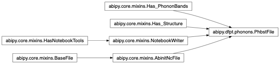
- to_string(verbose: int = 0) str[source]
String representation
- Parameters:
verbose – verbosity level.
- property qpoints
List of q-point objects.
- property phbands: PhononBands
- qindex(qpoint)[source]
Returns the index of the qpoint in the PhbstFile. Accepts integer, vector with reduced coordinates or
abipy.core.kpoints.Kpoint.
- qindex_qpoint(qpoint, is_non_analytical_direction=False)[source]
Returns (qindex, qpoint). Accepts integer, vector with reduced coordinates or
abipy.core.kpoints.Kpoint.
- get_phframe(qpoint, with_structure=True)[source]
Return a
pandas.DataFramewith the phonon frequencies at the given q-point and information on the crystal structure (used for convergence studies).- Parameters:
qpoint – integer, vector of reduced coordinates or
abipy.core.kpoints.Kpointobject.with_structure – True to add structural parameters.
- get_phmode(qpoint, branch)[source]
Returns the
PhononModewith the given qpoint and branch nu.- Parameters:
qpoint – Either a vector with the reduced components of the q-point or an integer giving the sequential index (C-convention).
branch – branch index (C-convention)
- Returns:
PhononModeinstance.
- yield_figs(**kwargs)[source]
This function generates a predefined list of matplotlib figures with minimal input from the user.
- class abipy.dfpt.phonons.PhononDos(mesh, values)[source]
Bases:
Function1DThis object stores the phonon density of states. An instance of
PhononDoshas amesh(numpy array with the points of the mesh) and another numpy array,values, with the DOS on the mesh.Note
mesh is given in eV, values are in states/eV.
- classmethod as_phdos(obj: Any, phdos_kwargs=None) PhononDos[source]
Return an instance of
abipy.dfpt.phonons.PhononDosfrom a generic obj. Supports:- instances of cls - files (string) that can be open with abiopen and that provide one of the following attributes: [`phdos`, `phbands`] - instances of |PhononBands|. - objects providing a ``phbands`` attribute.
- Parameters:
phdos_kwargs – optional dictionary with the options passed to
get_phdosto compute the phonon DOS.obj. (Used when obj is not already an instance of cls or when we have to compute the DOS from)
- plot_dos_idos(ax, what='d', exchange_xy=False, units='eV', **kwargs)[source]
Helper function to plot DOS/IDOS on the axis
ax.- Parameters:
ax –
matplotlib.axes.Axeswhat – string selecting the quantity to plot: “d” for DOS, “i” for IDOS. chars can be concatenated hence what=”id” plots both IDOS and DOS. (default “d”).
exchange_xy – True to exchange axis
units – Units for phonon plots. Possible values in (“eV”, “meV”, “Ha”, “cm-1”, “Thz”). Case-insensitive.
kwargs – Options passed to matplotlib plot method.
- Returns:
list of lines added to the plot.
- plotly_dos_idos(fig, what='d', trace_name=None, exchange_xy=False, units='eV', rcd=None, **kwargs)[source]
Helper function to plot DOS/IDOS on the figure
fig.- Parameters:
fig –
plotly.graph_objects.Figurewhat – string selecting the quantity to plot: “d” for DOS, “i” for IDOS. chars can be concatenated hence what=”id” plots both IDOS and DOS. (default “d”).
exchange_xy – True to exchange axis
units – Units for phonon plots. Possible values in (“eV”, “meV”, “Ha”, “cm-1”, “Thz”). Case-insensitive.
rcd – PlotlyRowColDesc object used when fig is not None to specify the (row, col) of the subplot in the grid.
kwargs – Passed to fig.add_scatter method.
- plot(units='eV', **kwargs) Any[source]
Plot Phonon DOS and IDOS on two distinct plots.
- Parameters:
units – Units for phonon plots. Possible values in (“eV”, “meV”, “Ha”, “cm-1”, “Thz”). Case-insensitive.
kwargs – Keyword arguments passed to
matplotlib.
Returns:
matplotlib.figure.FigureKeyword arguments controlling the display of the figure:
kwargs
Meaning
title
Title of the plot (Default: None).
show
True to show the figure (default: True).
savefig
“abc.png” or “abc.eps” to save the figure to a file.
size_kwargs
Dictionary with options passed to fig.set_size_inches e.g. size_kwargs=dict(w=3, h=4)
tight_layout
True to call fig.tight_layout (default: False)
ax_grid
True (False) to add (remove) grid from all axes in fig. Default: None i.e. fig is left unchanged.
ax_annotate
Add labels to subplots e.g. (a), (b). Default: False
fig_close
Close figure. Default: False.
plotly
Try to convert mpl figure to plotly.
- plotly(units='eV', **kwargs)[source]
Plot Phonon DOS and IDOS on two distinct plots.
- Parameters:
units – Units for phonon plots. Possible values in (“eV”, “meV”, “Ha”, “cm-1”, “Thz”). Case-insensitive.
kwargs – Keyword arguments passed to mod:plotly.
Returns:
plotly.graph_objects.FigureKeyword arguments controlling the display of the figure: ================ ==================================================================== kwargs Meaning ================ ==================================================================== title Title of the plot (Default: None). show True to show the figure (default: True). hovermode True to show the hover info (default: False) savefig “abc.png” , “abc.jpeg” or “abc.webp” to save the figure to a file. write_json Write plotly figure to write_json JSON file.
Inside jupyter-lab, one can right-click the write_json file from the file menu and open with “Plotly Editor”. Make some changes to the figure, then use the file menu to save the customized plotly plot. Requires jupyter labextension install jupyterlab-chart-editor. See https://github.com/plotly/jupyterlab-chart-editor
- renderer (str or None (default None)) –
A string containing the names of one or more registered renderers (separated by ‘+’ characters) or None. If None, then the default renderers specified in plotly.io.renderers.default are used. See https://plotly.com/python-api-reference/generated/plotly.graph_objects.Figure.html
config (dict) A dict of parameters to configure the figure. The defaults are set in plotly.js. chart_studio True to push figure to chart_studio server. Requires authenticatios.
Default: False.
- template Plotly template. See https://plotly.com/python/templates/
- [“plotly”, “plotly_white”, “plotly_dark”, “ggplot2”,
“seaborn”, “simple_white”, “none”]
Default is None that is the default template is used.
- get_internal_energy(tstart=5, tstop=300, num=50) Function1D[source]
Returns the internal energy, in eV, in the harmonic approximation for different temperatures Zero point energy is included.
- Parameters:
tstart – The starting value (in Kelvin) of the temperature mesh.
tstop – The end value (in Kelvin) of the mesh.
num (int) – optional Number of samples to generate. Default is 50.
Return:
abipy.core.func1d.Function1Dobject with U(T) + ZPE.
- get_entropy(tstart=5, tstop=300, num=50) Function1D[source]
Returns the entropy, in eV/K, in the harmonic approximation for different temperatures
- Parameters:
tstart – The starting value (in Kelvin) of the temperature mesh.
tstop – The end value (in Kelvin) of the mesh.
num (int) – optional Number of samples to generate. Default is 50.
Return:
abipy.core.func1d.Function1Dobject with S(T).
- get_free_energy(tstart=5, tstop=300, num=50) Function1D[source]
Returns the free energy, in eV, in the harmonic approximation for different temperatures Zero point energy is included.
- Parameters:
tstart – The starting value (in Kelvin) of the temperature mesh.
tstop – The end value (in Kelvin) of the mesh.
num (int) – optional Number of samples to generate. Default is 50.
Return:
abipy.core.func1d.Function1Dobject with F(T) = U(T) + ZPE - T x S(T)
- get_cv(tstart=5, tstop=300, num=50) Function1D[source]
Returns the constant-volume specific heat, in eV/K, in the harmonic approximation for different temperatures
- Parameters:
tstart – The starting value (in Kelvin) of the temperature mesh.
tstop – The end value (in Kelvin) of the mesh.
num (int) – optional Number of samples to generate. Default is 50.
Return:
abipy.core.func1d.Function1Dobject with C_v(T).
- plot_harmonic_thermo(tstart=5, tstop=300, num=50, units='eV', formula_units=None, quantities='all', fontsize=8, **kwargs) Any[source]
Plot thermodynamic properties from the phonon DOSes within the harmonic approximation.
- Parameters:
tstart – The starting value (in Kelvin) of the temperature mesh.
tstop – The end value (in Kelvin) of the mesh.
num – int, optional Number of samples to generate. Default is 50.
quantities – List of strings specifying the thermodynamic quantities to plot. Possible values: [“internal_energy”, “free_energy”, “entropy”, “c_v”].
units – eV for energies in ev/unit_cell, Jmol for results in J/mole.
formula_units – the number of formula units per unit cell. If unspecified, the thermodynamic quantities will be given on a per-unit-cell basis.
fontsize – Label and title fontsize.
Returns:
matplotlib.figure.FigureKeyword arguments controlling the display of the figure:
kwargs
Meaning
title
Title of the plot (Default: None).
show
True to show the figure (default: True).
savefig
“abc.png” or “abc.eps” to save the figure to a file.
size_kwargs
Dictionary with options passed to fig.set_size_inches e.g. size_kwargs=dict(w=3, h=4)
tight_layout
True to call fig.tight_layout (default: False)
ax_grid
True (False) to add (remove) grid from all axes in fig. Default: None i.e. fig is left unchanged.
ax_annotate
Add labels to subplots e.g. (a), (b). Default: False
fig_close
Close figure. Default: False.
plotly
Try to convert mpl figure to plotly.
- plotly_harmonic_thermo(tstart=5, tstop=300, num=50, units='eV', formula_units=None, quantities='all', fontsize=12, **kwargs)[source]
Plot thermodynamic properties from the phonon DOS within the harmonic approximation.
- Parameters:
tstart – The starting value (in Kelvin) of the temperature mesh.
tstop – The end value (in Kelvin) of the mesh.
num – int, optional Number of samples to generate. Default is 50.
quantities – List of strings specifying the thermodynamic quantities to plot. Possible values: [“internal_energy”, “free_energy”, “entropy”, “c_v”].
units – eV for energies in ev/unit_cell, Jmol for results in J/mole.
formula_units – the number of formula units per unit cell. If unspecified, the thermodynamic quantities will be given on a per-unit-cell basis.
fontsize – Label and title fontsize.
Returns
plotly.graph_objects.FigureKeyword arguments controlling the display of the figure: ================ ==================================================================== kwargs Meaning ================ ==================================================================== title Title of the plot (Default: None). show True to show the figure (default: True). hovermode True to show the hover info (default: False) savefig “abc.png” , “abc.jpeg” or “abc.webp” to save the figure to a file. write_json Write plotly figure to write_json JSON file.
Inside jupyter-lab, one can right-click the write_json file from the file menu and open with “Plotly Editor”. Make some changes to the figure, then use the file menu to save the customized plotly plot. Requires jupyter labextension install jupyterlab-chart-editor. See https://github.com/plotly/jupyterlab-chart-editor
- renderer (str or None (default None)) –
A string containing the names of one or more registered renderers (separated by ‘+’ characters) or None. If None, then the default renderers specified in plotly.io.renderers.default are used. See https://plotly.com/python-api-reference/generated/plotly.graph_objects.Figure.html
config (dict) A dict of parameters to configure the figure. The defaults are set in plotly.js. chart_studio True to push figure to chart_studio server. Requires authenticatios.
Default: False.
- template Plotly template. See https://plotly.com/python/templates/
- [“plotly”, “plotly_white”, “plotly_dark”, “ggplot2”,
“seaborn”, “simple_white”, “none”]
Default is None that is the default template is used.
- class abipy.dfpt.phonons.PhononDosPlotter(key_phdos=None, phdos_kwargs=None)[source]
Bases:
NotebookWriterClass for plotting multiple phonon DOSes.
Usage example:
plotter = PhononDosPlotter()
plotter.add_phdos("foo dos", "foo.nc")
plotter.add_phdos("bar dos", "bar.nc")
plotter.gridplot()
- add_phdos(label, phdos, phdos_kwargs=None) None[source]
Adds a DOS for plotting.
- Parameters:
label – label for the phonon DOS. Must be unique.
phdos –
abipy.dfpt.phonons.PhononDosobject.phdos_kwargs – optional dictionary with the options passed to get_phdos to compute the phonon DOS. Used when phdos is not already an instance of cls or when we have to compute the DOS from obj.
- combiplot(ax=None, units='eV', xlims=None, ylims=None, fontsize=8, **kwargs) Any[source]
Plot DOSes on the same figure. Use
gridplotto plot DOSes on different figures.- Parameters:
ax –
matplotlib.axes.Axesor None if a new figure should be created.units – Units for phonon plots. Possible values in (“eV”, “meV”, “Ha”, “cm-1”, “Thz”). Case-insensitive.
xlims – Set the data limits for the x-axis. Accept tuple e.g. (left, right) or scalar e.g. left. If left (right) is None, default values are used
ylims – y-axis limits.
fontsize – Legend and title fontsize.
Returns:
matplotlib.figure.FigureKeyword arguments controlling the display of the figure:
kwargs
Meaning
title
Title of the plot (Default: None).
show
True to show the figure (default: True).
savefig
“abc.png” or “abc.eps” to save the figure to a file.
size_kwargs
Dictionary with options passed to fig.set_size_inches e.g. size_kwargs=dict(w=3, h=4)
tight_layout
True to call fig.tight_layout (default: False)
ax_grid
True (False) to add (remove) grid from all axes in fig. Default: None i.e. fig is left unchanged.
ax_annotate
Add labels to subplots e.g. (a), (b). Default: False
fig_close
Close figure. Default: False.
plotly
Try to convert mpl figure to plotly.
- combiplotly(fig=None, units='eV', xlims=None, ylims=None, fontsize=8, **kwargs)[source]
Plot DOSes on the same plotly figure. Use
gridplotlyto plot DOSes on different figures.- Parameters:
fig – plotly figure or None if a new figure should be created.
units – Units for phonon plots. Possible values in (“eV”, “meV”, “Ha”, “cm-1”, “Thz”). Case-insensitive.
xlims – Set the data limits for the x-axis. Accept tuple e.g.
(left, right).ylims – Set the data limits for the y-axis. Accept tuple e.g.
(left, right).fontsize – Legend and title fontsize.
Returns:
plotly.graph_objects.FigureKeyword arguments controlling the display of the figure: ================ ==================================================================== kwargs Meaning ================ ==================================================================== title Title of the plot (Default: None). show True to show the figure (default: True). hovermode True to show the hover info (default: False) savefig “abc.png” , “abc.jpeg” or “abc.webp” to save the figure to a file. write_json Write plotly figure to write_json JSON file.
Inside jupyter-lab, one can right-click the write_json file from the file menu and open with “Plotly Editor”. Make some changes to the figure, then use the file menu to save the customized plotly plot. Requires jupyter labextension install jupyterlab-chart-editor. See https://github.com/plotly/jupyterlab-chart-editor
- renderer (str or None (default None)) –
A string containing the names of one or more registered renderers (separated by ‘+’ characters) or None. If None, then the default renderers specified in plotly.io.renderers.default are used. See https://plotly.com/python-api-reference/generated/plotly.graph_objects.Figure.html
config (dict) A dict of parameters to configure the figure. The defaults are set in plotly.js. chart_studio True to push figure to chart_studio server. Requires authenticatios.
Default: False.
- template Plotly template. See https://plotly.com/python/templates/
- [“plotly”, “plotly_white”, “plotly_dark”, “ggplot2”,
“seaborn”, “simple_white”, “none”]
Default is None that is the default template is used.
- gridplot(units='eV', xlims=None, ylims=None, fontsize=8, **kwargs) Any[source]
Plot multiple DOSes on a grid with matplotlib.
- Parameters:
units – eV for energies in ev/unit_cell, Jmol for results in J/mole.
xlims – Set the data limits for the x-axis. Accept tuple e.g.
(left, right)or scalar e.g.left. If left (right) is None, default values are usedfontsize – Axis_label and subtitle fontsize.
Returns:
matplotlib.figure.FigureKeyword arguments controlling the display of the figure:
kwargs
Meaning
title
Title of the plot (Default: None).
show
True to show the figure (default: True).
savefig
“abc.png” or “abc.eps” to save the figure to a file.
size_kwargs
Dictionary with options passed to fig.set_size_inches e.g. size_kwargs=dict(w=3, h=4)
tight_layout
True to call fig.tight_layout (default: False)
ax_grid
True (False) to add (remove) grid from all axes in fig. Default: None i.e. fig is left unchanged.
ax_annotate
Add labels to subplots e.g. (a), (b). Default: False
fig_close
Close figure. Default: False.
plotly
Try to convert mpl figure to plotly.
- gridplotly(units='eV', xlims=None, ylims=None, fontsize=12, **kwargs)[source]
Plot multiple DOSes on a grid with plotly.
- Parameters:
units – eV for energies in ev/unit_cell, Jmol for results in J/mole.
xlims – Set the data limits for the x-axis. Accept tuple e.g.
(left, right)fontsize – Axis_label and subtitle fontsize.
Returns:
plotly.graph_objects.FigureKeyword arguments controlling the display of the figure: ================ ==================================================================== kwargs Meaning ================ ==================================================================== title Title of the plot (Default: None). show True to show the figure (default: True). hovermode True to show the hover info (default: False) savefig “abc.png” , “abc.jpeg” or “abc.webp” to save the figure to a file. write_json Write plotly figure to write_json JSON file.
Inside jupyter-lab, one can right-click the write_json file from the file menu and open with “Plotly Editor”. Make some changes to the figure, then use the file menu to save the customized plotly plot. Requires jupyter labextension install jupyterlab-chart-editor. See https://github.com/plotly/jupyterlab-chart-editor
- renderer (str or None (default None)) –
A string containing the names of one or more registered renderers (separated by ‘+’ characters) or None. If None, then the default renderers specified in plotly.io.renderers.default are used. See https://plotly.com/python-api-reference/generated/plotly.graph_objects.Figure.html
config (dict) A dict of parameters to configure the figure. The defaults are set in plotly.js. chart_studio True to push figure to chart_studio server. Requires authenticatios.
Default: False.
- template Plotly template. See https://plotly.com/python/templates/
- [“plotly”, “plotly_white”, “plotly_dark”, “ggplot2”,
“seaborn”, “simple_white”, “none”]
Default is None that is the default template is used.
- plot_harmonic_thermo(tstart=5, tstop=300, num=50, units='eV', formula_units=1, quantities='all', fontsize=8, **kwargs) Any[source]
Plot thermodynamic properties from the phonon DOS within the harmonic approximation for all the files in the plotter with matplotlib.
- Parameters:
tstart – The starting value (in Kelvin) of the temperature mesh.
tstop – The end value (in Kelvin) of the mesh.
num – int, optional Number of samples to generate. Default is 50.
units – eV for energies in ev/unit_cell, Jmol for results in J/mole.
formula_units – the number of formula units per unit cell. If unspecified, the thermodynamic quantities will be given on a per-unit-cell basis.
quantities – List of strings specifying the thermodynamic quantities to plot. Possible values in [“internal_energy”, “free_energy”, “entropy”, “c_v”].
fontsize – Legend, axis_label and subtitles fontsize.
Returns:
matplotlib.figure.FigureKeyword arguments controlling the display of the figure:
kwargs
Meaning
title
Title of the plot (Default: None).
show
True to show the figure (default: True).
savefig
“abc.png” or “abc.eps” to save the figure to a file.
size_kwargs
Dictionary with options passed to fig.set_size_inches e.g. size_kwargs=dict(w=3, h=4)
tight_layout
True to call fig.tight_layout (default: False)
ax_grid
True (False) to add (remove) grid from all axes in fig. Default: None i.e. fig is left unchanged.
ax_annotate
Add labels to subplots e.g. (a), (b). Default: False
fig_close
Close figure. Default: False.
plotly
Try to convert mpl figure to plotly.
- plotly_harmonic_thermo(tstart=5, tstop=300, num=50, units='eV', formula_units=1, quantities='all', fontsize=12, **kwargs)[source]
Plot thermodynamic properties from the phonon DOS within the harmonic approximation for all the files in the plotter with plotly.
- Parameters:
tstart – The starting value (in Kelvin) of the temperature mesh.
tstop – The end value (in Kelvin) of the mesh.
num – int, optional Number of samples to generate. Default is 50.
units – eV for energies in ev/unit_cell, Jmol for results in J/mole.
formula_units – the number of formula units per unit cell. If unspecified, the thermodynamic quantities will be given on a per-unit-cell basis.
quantities – List of strings specifying the thermodynamic quantities to plot. Possible values in [“internal_energy”, “free_energy”, “entropy”, “c_v”].
fontsize – Legend, axis_label and subtitle fontsize.
Returns:
plotly.graph_objects.FigureKeyword arguments controlling the display of the figure: ================ ==================================================================== kwargs Meaning ================ ==================================================================== title Title of the plot (Default: None). show True to show the figure (default: True). hovermode True to show the hover info (default: False) savefig “abc.png” , “abc.jpeg” or “abc.webp” to save the figure to a file. write_json Write plotly figure to write_json JSON file.
Inside jupyter-lab, one can right-click the write_json file from the file menu and open with “Plotly Editor”. Make some changes to the figure, then use the file menu to save the customized plotly plot. Requires jupyter labextension install jupyterlab-chart-editor. See https://github.com/plotly/jupyterlab-chart-editor
- renderer (str or None (default None)) –
A string containing the names of one or more registered renderers (separated by ‘+’ characters) or None. If None, then the default renderers specified in plotly.io.renderers.default are used. See https://plotly.com/python-api-reference/generated/plotly.graph_objects.Figure.html
config (dict) A dict of parameters to configure the figure. The defaults are set in plotly.js. chart_studio True to push figure to chart_studio server. Requires authenticatios.
Default: False.
- template Plotly template. See https://plotly.com/python/templates/
- [“plotly”, “plotly_white”, “plotly_dark”, “ggplot2”,
“seaborn”, “simple_white”, “none”]
Default is None that is the default template is used.
- ipw_harmonic_thermo()[source]
Return an ipython widget with controllers to plot thermodynamic properties from the phonon DOS within the harmonic approximation.
- yield_figs(**kwargs)[source]
This function generates a predefined list of matplotlib figures with minimal input from the user.
- class abipy.dfpt.phonons.PhdosReader(path)[source]
Bases:
ETSF_ReaderThis object reads data from the PHDOS.nc file produced by anaddb.
Note
Frequencies are in eV, DOSes are in states/eV per unit cell.
- structure()[source]
abipy.core.structure.Structureobject.
- read_pjdos_atdir()[source]
Return [natom, three, nomega] array with Phonon DOS projected over atoms and cartesian directions.
- read_phdos() PhononDos[source]
Return
abipy.dfpt.phonons.PhononDosobject with the total phonon DOS
- read_pjdos_symbol_xyz_dict()[source]
Return
OrderedDictmapping element symbol –> [3, nomega] array with the the phonon DOSes summed over atom-types and decomposed along the three cartesian directions.
- read_pjdos_symbol_dict()[source]
Ordered dictionary mapping element symbol –>
abipy.dfpt.phonons.PhononDoswhere PhononDos is the contribution to the total DOS summed over atoms with chemical symbolsymbol.
- read_msq_dos()[source]
Read generalized DOS with MSQ displacement tensor in cartesian coords.
Return:
abipy.dfpt.msqdos.MsqDosobject.
- class abipy.dfpt.phonons.PhdosFile(filepath: str)[source]
Bases:
AbinitNcFile,Has_Structure,NotebookWriterContainer object storing the different DOSes stored in the PHDOS.nc file produced by anaddb. Provides helper function to visualize/extract data.
Inheritance Diagram
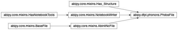
- params()[source]
OrderedDictwith the convergence parameters Used to constructpandas.DataFrame.
- to_string(verbose: int = 0) str[source]
Human-readable string with useful information such as structure…
- Parameters:
verbose – Verbosity level.
- structure()[source]
abipy.core.structure.Structureobject.
- phdos()[source]
abipy.dfpt.phonons.PhononDosobject.
- pjdos_symbol()[source]
Ordered dictionary mapping element symbol –> PhononDos where PhononDos is the contribution to the total DOS summed over atoms with chemical symbol symbol.
- msqd_dos()[source]
abipy.dfpt.msqdos.MsqDosobject with Mean square displacement tensor in cartesian coords. Allows one to calculate Debye Waller factors by integration with 1/omega and the Bose-Einstein factor.
- plot_pjdos_type(units='eV', stacked=True, colormap='jet', alpha=0.7, exchange_xy=False, ax=None, xlims=None, ylims=None, fontsize=12, **kwargs) Any[source]
Plot type-projected phonon DOS with matplotlib.
- Parameters:
ax –
matplotlib.axes.Axesor None if a new figure should be created.stacked – True if DOS partial contributions should be stacked on top of each other.
units – Units for phonon plots. Possible values in (“eV”, “meV”, “Ha”, “cm-1”, “Thz”). Case-insensitive.
colormap – Have a look at the colormaps here and decide which one you’d like:
alpha – The alpha blending value, between 0 (transparent) and 1 (opaque).
exchange_xy – True to exchange x-y axis.
xlims – Set the data limits for the x-axis. Accept tuple e.g.
(left, right)or scalar e.g.left. If left (right) is None, default values are used.ylims – y-axis limits.
fontsize – legend and title fontsize.
Returns:
matplotlib.figure.FigureKeyword arguments controlling the display of the figure:
kwargs
Meaning
title
Title of the plot (Default: None).
show
True to show the figure (default: True).
savefig
“abc.png” or “abc.eps” to save the figure to a file.
size_kwargs
Dictionary with options passed to fig.set_size_inches e.g. size_kwargs=dict(w=3, h=4)
tight_layout
True to call fig.tight_layout (default: False)
ax_grid
True (False) to add (remove) grid from all axes in fig. Default: None i.e. fig is left unchanged.
ax_annotate
Add labels to subplots e.g. (a), (b). Default: False
fig_close
Close figure. Default: False.
plotly
Try to convert mpl figure to plotly.
- plotly_pjdos_type(units='eV', stacked=True, exchange_xy=False, fig=None, xlims=None, ylims=None, fontsize=12, **kwargs)[source]
Plot type-projected phonon DOS with plotly.
- Parameters:
fig – plotly figure or None if a new figure should be created.
stacked – True if DOS partial contributions should be stacked on top of each other.
units – Units for phonon plots. Possible values in (“eV”, “meV”, “Ha”, “cm-1”, “Thz”). Case-insensitive.
exchange_xy – True to exchange x-y axis.
xlims – Set the data limits for the x-axis. Accept tuple e.g.
(left, right).ylims – Set the data limits for the y-axis. Accept tuple e.g.
(left, right).fontsize – legend and title fontsize.
Returns:
plotly.graph_objects.FigureKeyword arguments controlling the display of the figure: ================ ==================================================================== kwargs Meaning ================ ==================================================================== title Title of the plot (Default: None). show True to show the figure (default: True). hovermode True to show the hover info (default: False) savefig “abc.png” , “abc.jpeg” or “abc.webp” to save the figure to a file. write_json Write plotly figure to write_json JSON file.
Inside jupyter-lab, one can right-click the write_json file from the file menu and open with “Plotly Editor”. Make some changes to the figure, then use the file menu to save the customized plotly plot. Requires jupyter labextension install jupyterlab-chart-editor. See https://github.com/plotly/jupyterlab-chart-editor
- renderer (str or None (default None)) –
A string containing the names of one or more registered renderers (separated by ‘+’ characters) or None. If None, then the default renderers specified in plotly.io.renderers.default are used. See https://plotly.com/python-api-reference/generated/plotly.graph_objects.Figure.html
config (dict) A dict of parameters to configure the figure. The defaults are set in plotly.js. chart_studio True to push figure to chart_studio server. Requires authenticatios.
Default: False.
- template Plotly template. See https://plotly.com/python/templates/
- [“plotly”, “plotly_white”, “plotly_dark”, “ggplot2”,
“seaborn”, “simple_white”, “none”]
Default is None that is the default template is used.
- plot_pjdos_cartdirs_type(units='eV', stacked=True, colormap='jet', alpha=0.7, xlims=None, ylims=None, ax_list=None, fontsize=8, **kwargs) Any[source]
Plot type-projected phonon DOS decomposed along the three cartesian directions. Three rows for each cartesian direction. Each row shows the contribution of each atomic type + Total Phonon DOS.
- Parameters:
units – Units for phonon plots. Possible values in (“eV”, “meV”, “Ha”, “cm-1”, “Thz”). Case-insensitive.
stacked – True if DOS partial contributions should be stacked on top of each other.
colormap –
Have a look at the colormaps here and decide which one you’d like:
alpha – The alpha blending value, between 0 (transparent) and 1 (opaque)
xlims – Set the data limits for the x-axis. Accept tuple e.g.
(left, right)or scalar e.g.left. If left (right) is None, default values are usedylims – y-axis limits.
ax_list – List of
matplotlib.axes.Axesor None if a new figure should be created.fontsize – Legend and label fontsize.
Returns:
matplotlib.figure.Figure.Keyword arguments controlling the display of the figure:
kwargs
Meaning
title
Title of the plot (Default: None).
show
True to show the figure (default: True).
savefig
“abc.png” or “abc.eps” to save the figure to a file.
size_kwargs
Dictionary with options passed to fig.set_size_inches e.g. size_kwargs=dict(w=3, h=4)
tight_layout
True to call fig.tight_layout (default: False)
ax_grid
True (False) to add (remove) grid from all axes in fig. Default: None i.e. fig is left unchanged.
ax_annotate
Add labels to subplots e.g. (a), (b). Default: False
fig_close
Close figure. Default: False.
plotly
Try to convert mpl figure to plotly.
- plot_pjdos_cartdirs_site(view='inequivalent', units='eV', stacked=True, colormap='jet', alpha=0.7, xlims=None, ylims=None, ax_list=None, fontsize=8, verbose=0, **kwargs) Any[source]
Plot phonon PJDOS for each atom in the unit cell. By default, only “inequivalent” atoms are shown.
- Parameters:
view – “inequivalent” to show only inequivalent atoms. “all” for all sites.
units – Units for phonon plots. Possible values in (“eV”, “meV”, “Ha”, “cm-1”, “Thz”). Case-insensitive.
stacked – True if DOS partial contributions should be stacked on top of each other.
colormap – matplotlib colormap.
alpha – The alpha blending value, between 0 (transparent) and 1 (opaque)
xlims – Set the data limits for the x-axis. Accept tuple e.g.
(left, right)or scalar e.g.left. If left (right) is None, default values are used.ylims – Set the data limits for the y-axis. Accept tuple e.g.
(left, right)or scalar e.g.left. If left (right) is None, default values are usedax_list – List of
matplotlib.axes.Axesor None if a new figure should be created.fontsize – Legend and title fontsize.
verbose – Verbosity level.
Returns:
matplotlib.figure.FigureKeyword arguments controlling the display of the figure:
kwargs
Meaning
title
Title of the plot (Default: None).
show
True to show the figure (default: True).
savefig
“abc.png” or “abc.eps” to save the figure to a file.
size_kwargs
Dictionary with options passed to fig.set_size_inches e.g. size_kwargs=dict(w=3, h=4)
tight_layout
True to call fig.tight_layout (default: False)
ax_grid
True (False) to add (remove) grid from all axes in fig. Default: None i.e. fig is left unchanged.
ax_annotate
Add labels to subplots e.g. (a), (b). Default: False
fig_close
Close figure. Default: False.
plotly
Try to convert mpl figure to plotly.
- yield_figs(**kwargs)[source]
This function generates a predefined list of matplotlib figures with minimal input from the user. Used in abiview.py to get a quick look at the results.
- yield_plotly_figs(**kwargs)[source]
This function generates a predefined list of plotly figures with minimal input from the user. Used in abiview.py to get a quick look at the results.
phtk Module
Phonon Toolkit: This module gathers low-level tools to operate on phonons.
- abipy.dfpt.phtk.get_dyn_mat_eigenvec(phdispl, structure, amu=None, amu_symbol=None) ndarray[source]
Converts the phonon displacements to the orthonormal eigenvectors of the dynamical matrix. Small discrepancies with the original values may be expected due to the different values of the atomic masses in abinit and pymatgen.
Note
These eigenvectors are orthonormalized and should be very close to the ones computed by Abinit in a.u. Note, however, that the output vectors are given in atomic units so dividing then by the sqrt(Mass) won’t give the dipl_cart used in PhononBands that are in Angstrom.
- Parameters:
phdispl – a numpy array containing the displacements in cartesian coordinates. The last index should have size 3*(num atoms), but the rest of the shape is arbitrary. If qpts is not None the first dimension should match the q points.
structure –
abipy.core.structure.Structureobject.amu – dictionary that associates the atomic numbers present in the structure to the values of the atomic mass units used for the calculation. Incompatible with amu_sumbol. If None and amu_symbol is None, values from pymatgen will be used. Note that this will almost always lead to inaccuracies in the conversion.
amu_symbol – dictionary that associates the symbol present in the structure to the values of the atomic mass units used for the calculation. Incompatible with amu. If None and amu_symbol is None, values from pymatgen will be used. that this will almost always lead to inaccuracies in the conversion.
- Returns:
A
numpy.ndarrayof the same shape as phdispl containing the eigenvectors of the dynamical matrix
- abipy.dfpt.phtk.match_eigenvectors(v1, v2) ndarray[source]
Given two list of vectors, returns the pair matching based on the complex scalar product. Returns the indices of the second list that match the vectors of the first list in ascending order.
- class abipy.dfpt.phtk.NonAnalyticalPh(structure, directions, phfreqs, phdispl_cart, amu=None)[source]
Bases:
Has_StructurePhonon data at gamma including non analytical contributions Usually read from anaddb.nc
- classmethod from_file(filepath: str) NonAnalyticalPh[source]
Reads the non analytical directions, frequencies and displacements from the nc file specified (usually anaddb.nc) Non existence of displacements is accepted for compatibility with abinit 8.0.6 Raises an error if the other values are not present in the netcdf file.
- classmethod from_ncreader(nc_reader) NonAnalyticalPh[source]
Build the object from a NetcdfReader.
- dyn_mat_eigenvect()[source]
[ndirection, 3*natom, 3*natom] array with the orthonormal eigenvectors of the dynamical matrix. in Cartesian coordinates.
- property structure
abipy.core.structure.Structureobject.
- index_direction(direction, cartesian=False) int[source]
Returns: the index of direction. Raises: ValueError if not found.
- Parameters:
direction – a 3 element list indicating the direction. Can be a generic vector
cartesian – if True the direction are already in cartesian coordinates, if False it will be converted to match the internal description of the directions.
- has_direction(direction, cartesian=False) bool[source]
Checks if the input direction is among those available.
- Parameters:
direction – a 3 element list indicating the direction. Can be a generic vector
cartesian – if True the direction are already in cartesian coordinates, if False it will be converted to match the internal description of the directions.
- abipy.dfpt.phtk.open_file_phononwebsite(filename, port=8000, website='http://henriquemiranda.github.io/phononwebsite', host='localhost', browser=None)[source]
Take a file, detect the type and open it on the phonon website Based on a similar function in <https://github.com/henriquemiranda/phononwebsite/phononweb.py>
- Parameters:
filename – file with phonon data in phononwebsite format.
port – Initial port.
website – Website URL
host – localhost name.
browser – Open webpage in
browser. Use default if $BROWSER if None.
qha Module
- class abipy.dfpt.qha.AbstractQHA(structures, energies, eos_name='vinet', pressure=0)[source]
Bases:
objectAbstract class for the quasi-harmonic approximation analysis. Provides some basic methods and plotting utils, plus a converter to write input files for phonopy-qha or to generate an instance of phonopy.qha.core.QHA. These can be used to obtain other quantities and plots. Does not include electronic entropic contributions for metals.
- fit_energies(tstart=0, tstop=800, num=100)[source]
Performs a fit of the energies as a function of the volume at different temperatures.
- Parameters:
tstart – The starting value (in Kelvin) of the temperature mesh.
tstop – The end value (in Kelvin) of the mesh.
num – int, optional Number of samples to generate. Default is 100.
- Returns:
namedtuple with the following attributes:
tot_en: numpy array with shape (nvols, num) with the energies used for the fit
fits: list of subclasses of pymatgen.analysis.eos.EOSBase, depending on the type of
    eos chosen. Contains the fit for the energies at the different temperatures.
min_en: numpy array with the minimum energies for the list of temperatures
min_vol: numpy array with the minimum volumes for the list of temperatures
temp: numpy array with the temperatures considered
- abstract get_vib_free_energies(tstart=0, tstop=800, num=100)[source]
Generates the vibrational free energy corresponding to all the structures.
- Parameters:
tstart – The starting value (in Kelvin) of the temperature mesh.
tstop – The end value (in Kelvin) of the mesh.
num – int, optional Number of samples to generate. Default is 100.
Returns: A numpy array of num values of the vibrational contribution to the free energy
- abstract get_thermodynamic_properties(tstart=0, tstop=800, num=100)[source]
Generates all the thermodynamic properties corresponding to all the volumes.
- Parameters:
tstart – The starting value (in Kelvin) of the temperature mesh.
tstop – The end value (in Kelvin) of the mesh.
num – int, optional Number of samples to generate. Default is 100.
- Returns:
tmesh: numpy array with the list of temperatures. Shape (num). cv: constant-volume specific heat, in eV/K. Shape (nvols, num). free_energy: free energy, in eV. Shape (nvols, num). entropy: entropy, in eV/K. Shape (nvols, num). zpe: zero point energy in eV. Shape (nvols).
- Return type:
namedtuple with the following attributes for all the volumes
- set_eos(eos_name: str) None[source]
Set the EOS model used for the fit.
- Parameters:
eos_name – string indicating the expression used to fit the energies. See pymatgen.analysis.eos.EOS.
- plot_energies(tstart=0, tstop=800, num=10, ax=None, **kwargs) Any[source]
Plots the energies as a function of volume at different temperatures.
- Parameters:
tstart – The starting value (in Kelvin) of the temperature mesh.
tstop – The end value (in Kelvin) of the mesh.
num – int, optional Number of samples to generate. Default is 10.
ax –
matplotlib.axes.Axesor None if a new figure should be created.
Returns:
matplotlib.figure.FigureKeyword arguments controlling the display of the figure:
kwargs
Meaning
title
Title of the plot (Default: None).
show
True to show the figure (default: True).
savefig
“abc.png” or “abc.eps” to save the figure to a file.
size_kwargs
Dictionary with options passed to fig.set_size_inches e.g. size_kwargs=dict(w=3, h=4)
tight_layout
True to call fig.tight_layout (default: False)
ax_grid
True (False) to add (remove) grid from all axes in fig. Default: None i.e. fig is left unchanged.
ax_annotate
Add labels to subplots e.g. (a), (b). Default: False
fig_close
Close figure. Default: False.
plotly
Try to convert mpl figure to plotly.
- get_thermal_expansion_coeff(tstart=0, tstop=800, num=100, tref=None, method=None) Function1D[source]
Calculates the thermal expansion coefficient as a function of temperature, using finite difference on the fitted values of the volume as a function of temperature.
- Parameters:
tstart – The starting value (in Kelvin) of the temperature mesh.
tstop – The end value (in Kelvin) of the mesh.
tref – The reference temperature (in Kelvin) used to compute the thermal expansion coefficient 1/V(tref) * dV(T)/dT. (If tref is not available, it uses 1/V(T) * dV(T)/dT instead.)
num – int, optional Number of samples to generate. Default is 100.
Returns:
abipy.core.func1d.Function1D
- plot_thermal_expansion_coeff(tstart=0, tstop=800, num=100, tref=None, ax=None, **kwargs) Any[source]
Plots the thermal expansion coefficient as a function of the temperature.
- Parameters:
tstart – The starting value (in Kelvin) of the temperature mesh.
tstop – The end value (in Kelvin) of the mesh.
tref – The reference temperature (in Kelvin) used to compute the thermal expansion coefficient 1/V(tref) * dV(T)/dT. (If tref is not available, it uses 1/V(T) * dV(T)/dT instead.)
num – int, optional Number of samples to generate. Default is 100.
ax –
matplotlib.axes.Axesor None if a new figure should be created.
Returns:
matplotlib.figure.FigureKeyword arguments controlling the display of the figure:
kwargs
Meaning
title
Title of the plot (Default: None).
show
True to show the figure (default: True).
savefig
“abc.png” or “abc.eps” to save the figure to a file.
size_kwargs
Dictionary with options passed to fig.set_size_inches e.g. size_kwargs=dict(w=3, h=4)
tight_layout
True to call fig.tight_layout (default: False)
ax_grid
True (False) to add (remove) grid from all axes in fig. Default: None i.e. fig is left unchanged.
ax_annotate
Add labels to subplots e.g. (a), (b). Default: False
fig_close
Close figure. Default: False.
plotly
Try to convert mpl figure to plotly.
- plot_vol_vs_t(tstart=0, tstop=800, num=100, ax=None, **kwargs) Any[source]
Plot the volume as a function of the temperature.
- Parameters:
tstart – The starting value (in Kelvin) of the temperature mesh.
tstop – The end value (in Kelvin) of the mesh.
num – int, optional Number of samples to generate. Default is 100.
ax –
matplotlib.axes.Axesor None if a new figure should be created.
Returns:
matplotlib.figure.FigureKeyword arguments controlling the display of the figure:
kwargs
Meaning
title
Title of the plot (Default: None).
show
True to show the figure (default: True).
savefig
“abc.png” or “abc.eps” to save the figure to a file.
size_kwargs
Dictionary with options passed to fig.set_size_inches e.g. size_kwargs=dict(w=3, h=4)
tight_layout
True to call fig.tight_layout (default: False)
ax_grid
True (False) to add (remove) grid from all axes in fig. Default: None i.e. fig is left unchanged.
ax_annotate
Add labels to subplots e.g. (a), (b). Default: False
fig_close
Close figure. Default: False.
plotly
Try to convert mpl figure to plotly.
- get_abc(tstart=0, tstop=800, num=100)[source]
Plots the thermal expansion coefficient as a function of the temperature.
- Parameters:
tstart – The starting value (in Kelvin) of the temperature mesh.
tstop – The end value (in Kelvin) of the mesh.
tref – The reference temperature (in Kelvin) used to compute the thermal expansion coefficient 1/V(tref) * dV(T)/dT. (If tref is not available, it uses 1/V(T) * dV(T)/dT instead.)
num – int, optional Number of samples to generate. Default is 100.
ax –
matplotlib.axes.Axesor None if a new figure should be created.
Returns:
matplotlib.figure.Figure
- get_angles(tstart=0, tstop=800, num=100)[source]
Plots the thermal expansion coefficient as a function of the temperature.
- Parameters:
tstart – The starting value (in Kelvin) of the temperature mesh.
tstop – The end value (in Kelvin) of the mesh.
tref – The reference temperature (in Kelvin) used to compute the thermal expansion coefficient 1/V(tref) * dV(T)/dT. (If tref is not available, it uses 1/V(T) * dV(T)/dT instead.)
num – int, optional Number of samples to generate. Default is 100.
ax –
matplotlib.axes.Axesor None if a new figure should be created.
Returns:
matplotlib.figure.Figure
- plot_thermal_expansion_coeff_abc(tstart=0, tstop=800, num=100, tref=None, ax=None, **kwargs) Any[source]
Plots the thermal expansion coefficient as a function of the temperature.
- Parameters:
tstart – The starting value (in Kelvin) of the temperature mesh.
tstop – The end value (in Kelvin) of the mesh.
tref – The reference temperature (in Kelvin) used to compute the thermal expansion coefficient 1/V(tref) * dV(T)/dT. (If tref is not available, it uses 1/V(T) * dV(T)/dT instead.)
num – int, optional Number of samples to generate. Default is 100.
ax –
matplotlib.axes.Axesor None if a new figure should be created.
Returns:
matplotlib.figure.FigureKeyword arguments controlling the display of the figure:
kwargs
Meaning
title
Title of the plot (Default: None).
show
True to show the figure (default: True).
savefig
“abc.png” or “abc.eps” to save the figure to a file.
size_kwargs
Dictionary with options passed to fig.set_size_inches e.g. size_kwargs=dict(w=3, h=4)
tight_layout
True to call fig.tight_layout (default: False)
ax_grid
True (False) to add (remove) grid from all axes in fig. Default: None i.e. fig is left unchanged.
ax_annotate
Add labels to subplots e.g. (a), (b). Default: False
fig_close
Close figure. Default: False.
plotly
Try to convert mpl figure to plotly.
- plot_abc_vs_t(tstart=0, tstop=800, num=100, tref=None, ax=None, **kwargs) Any[source]
Plots the thermal expansion coefficient as a function of the temperature.
- Parameters:
tstart – The starting value (in Kelvin) of the temperature mesh.
tstop – The end value (in Kelvin) of the mesh.
tref – The reference temperature (in Kelvin) used to compute the thermal expansion coefficient 1/V(tref) * dV(T)/dT. (If tref is not available, it uses 1/V(T) * dV(T)/dT instead.)
num – int, optional Number of samples to generate. Default is 100.
ax –
matplotlib.axes.Axesor None if a new figure should be created.
Returns:
matplotlib.figure.FigureKeyword arguments controlling the display of the figure:
kwargs
Meaning
title
Title of the plot (Default: None).
show
True to show the figure (default: True).
savefig
“abc.png” or “abc.eps” to save the figure to a file.
size_kwargs
Dictionary with options passed to fig.set_size_inches e.g. size_kwargs=dict(w=3, h=4)
tight_layout
True to call fig.tight_layout (default: False)
ax_grid
True (False) to add (remove) grid from all axes in fig. Default: None i.e. fig is left unchanged.
ax_annotate
Add labels to subplots e.g. (a), (b). Default: False
fig_close
Close figure. Default: False.
plotly
Try to convert mpl figure to plotly.
- plot_angle_vs_t(tstart=0, tstop=800, num=100, tref=None, ax=None, **kwargs) Any[source]
Plots the thermal expansion coefficient as a function of the temperature.
- Parameters:
tstart – The starting value (in Kelvin) of the temperature mesh.
tstop – The end value (in Kelvin) of the mesh.
tref – The reference temperature (in Kelvin) used to compute the thermal expansion coefficient 1/V(tref) * dV(T)/dT. (If tref is not available, it uses 1/V(T) * dV(T)/dT instead.)
num – int, optional Number of samples to generate. Default is 100.
ax –
matplotlib.axes.Axesor None if a new figure should be created.
Returns:
matplotlib.figure.FigureKeyword arguments controlling the display of the figure:
kwargs
Meaning
title
Title of the plot (Default: None).
show
True to show the figure (default: True).
savefig
“abc.png” or “abc.eps” to save the figure to a file.
size_kwargs
Dictionary with options passed to fig.set_size_inches e.g. size_kwargs=dict(w=3, h=4)
tight_layout
True to call fig.tight_layout (default: False)
ax_grid
True (False) to add (remove) grid from all axes in fig. Default: None i.e. fig is left unchanged.
ax_annotate
Add labels to subplots e.g. (a), (b). Default: False
fig_close
Close figure. Default: False.
plotly
Try to convert mpl figure to plotly.
- plot_phbs(phbands, temperatures=None, t_max=1000, colormap='plasma', **kwargs) Any[source]
Given a list of
abipy.dfpt.phonons.PhononBandsplots the band structures with a color depending on the temperature using aabipy.dfpt.phonons.PhononBandsPlotter. If temperatures are not given they will be deduced inverting the dependence of volume with respect to the temperature. If a unique volume could not be identified an error will be raised.- Parameters:
phbands – list of
abipy.dfpt.phonons.PhononBandsobjects.temperatures – list of temperatures.
t_max – maximum temperature considered for plotting.
colormap – matplotlib color map.
Returns:
matplotlib.figure.FigureKeyword arguments controlling the display of the figure:
kwargs
Meaning
title
Title of the plot (Default: None).
show
True to show the figure (default: True).
savefig
“abc.png” or “abc.eps” to save the figure to a file.
size_kwargs
Dictionary with options passed to fig.set_size_inches e.g. size_kwargs=dict(w=3, h=4)
tight_layout
True to call fig.tight_layout (default: False)
ax_grid
True (False) to add (remove) grid from all axes in fig. Default: None i.e. fig is left unchanged.
ax_annotate
Add labels to subplots e.g. (a), (b). Default: False
fig_close
Close figure. Default: False.
plotly
Try to convert mpl figure to plotly.
- get_vol_at_t(t) float[source]
Calculates the volume corresponding to a specific temperature.
- Parameters:
t – temperature in K
Returns: The volume in Ang^3.
- get_t_for_vols(vols, t_max=1000) list[float][source]
Find the temperatures corresponding to a specific volume. The search is performed interpolating the V(T) dependence with a spline and finding the roots with of V(t) - v. It may return more than one temperature for a volume in case of non monotonic behavior.
- Parameters:
vols – list of volumes
t_max – maximum temperature considered for the fit
- Returns:
A list of lists of temperatures. For each volume more than one temperature can be identified.
- write_phonopy_qha_inputs(tstart=0, tstop=2100, num=211, path=None) None[source]
Writes nvols thermal_properties-i.yaml files that can be used as inputs for phonopy-qha. Notice that phonopy apparently requires the value of the 300 K temperature to be present in the list. Choose the values of tstart, tstop and num to satisfy this condition.
- Parameters:
tstart – The starting value (in Kelvin) of the temperature mesh.
tstop – The end value (in Kelvin) of the mesh.
num – int, optional Number of samples to generate. Default is 211.
path – a path to a folder where the files will be stored
- get_phonopy_qha(tstart=0, tstop=2100, num=211, eos='vinet', t_max=None, energy_plot_factor=None, pressure=None)[source]
Creates an instance of phonopy.qha.core.QHA that can be used generate further plots and output data. The object is returned right after the construction. The “run()” method should be executed before getting results and plots. Notice that phonopy apparently requires the value of the 300 K temperature to be present in the list. Choose the values of tstart, tstop and num to satisfy this condition.
- Parameters:
tstart – The starting value (in Kelvin) of the temperature mesh.
tstop – The end value (in Kelvin) of the mesh.
num – int, optional Number of samples to generate. Default is 211.
eos – the expression used to fit the energies in phonopy. Possible values are “vinet”, “murnaghan” and “birch_murnaghan”. Passed to phonopy’s QHA.
t_max – maximum temperature. Passed to phonopy’s QHA.
energy_plot_factor – factor multiplying the energies. Passed to phonopy’s QHA.
pressure – pressure value, passed to phonopy.
Returns: An instance of phonopy.qha.core.QHA
- class abipy.dfpt.qha.QHA(structures, phdoses, energies, eos_name='vinet', pressure=0)[source]
Bases:
AbstractQHAObject to extract results in the quasi-harmonic approximation from electronic and phonon calculations at different volumes. Provides some basic methods and plotting utils, plus a converter to write input files for phonopy-qha or to generate an instance of phonopy.qha.core.QHA. These can be used to obtain other quantities and plots. Does not include electronic entropic contributions for metals.
Inheritance Diagram

- classmethod from_files(gsr_paths, phdos_paths)[source]
Creates an instance of QHA from a list of GSR files and a list of PHDOS.nc files. The list should have the same size and the volumes should match.
- Parameters:
gsr_paths – list of paths to GSR files.
phdos_paths – list of paths to PHDOS.nc files.
Returns: A new instance of QHA
- get_vib_free_energies(tstart=0, tstop=800, num=100) ndarray[source]
Generates the vibrational free energy from the phonon DOS.
- Parameters:
tstart – The starting value (in Kelvin) of the temperature mesh.
tstop – The end value (in Kelvin) of the mesh.
num – int, optional Number of samples to generate. Default is 100.
Returns: A numpy array of num values of the vibrational contribution to the free energy
- get_thermodynamic_properties(tstart=0, tstop=800, num=100)[source]
Generates all the thermodynamic properties corresponding to all the volumes using the phonon DOS.
- Parameters:
tstart – The starting value (in Kelvin) of the temperature mesh.
tstop – The end value (in Kelvin) of the mesh.
num – int, optional Number of samples to generate. Default is 100.
- Returns:
tmesh: numpy array with the list of temperatures. Shape (num). cv: constant-volume specific heat, in eV/K. Shape (nvols, num). free_energy: free energy, in eV. Shape (nvols, num). entropy: entropy, in eV/K. Shape (nvols, num). zpe: zero point energy in eV. Shape (nvols).
- Return type:
namedtuple with the following attributes for all the volumes
- class abipy.dfpt.qha.QHA3PF(structures, phdoses, energies, ind_doses, eos_name='vinet', pressure=0, fit_degree=2)[source]
Bases:
AbstractQHAObject to extract results in the quasi-harmonic approximation from several electronic energies at different volumes and three phonon calculations. Provides some basic methods and plotting utils, plus a converter to write input files for phonopy-qha or to generate an instance of phonopy.qha.core.QHA. These can be used to obtain other quantities and plots. Does not include electronic entropic contributions for metals.
Inheritance Diagram

- classmethod from_files(gsr_paths, phdos_paths, ind_doses) QHA3PF[source]
Creates an instance of QHA from a list of GSR files and a list of PHDOS.nc files. The list should have the same size and the volumes should match.
- Parameters:
gsr_paths – list of paths to GSR files.
phdos_paths – list of paths to three PHDOS.nc files.
ind_doses – list of three values indicating, for each of the three phdoses, the index of the corresponding gsr_file in “gsr_paths”.
Returns: A new instance of QHA3PF
- get_thermodynamic_properties(tstart=0, tstop=800, num=100)[source]
Generates all the thermodynamic properties corresponding to all the volumes using the phonon DOS.
- Parameters:
tstart – The starting value (in Kelvin) of the temperature mesh.
tstop – The end value (in Kelvin) of the mesh.
num – int, optional Number of samples to generate. Default is 100.
- Returns:
tmesh: numpy array with the list of temperatures. Shape (num). cv: constant-volume specific heat, in eV/K. Shape (nvols, num). free_energy: free energy, in eV. Shape (nvols, num). entropy: entropy, in eV/K. Shape (nvols, num). zpe: zero point energy in eV. Shape (nvols).
- Return type:
namedtuple with the following attributes for all the volumes
- get_vib_free_energies(tstart=0, tstop=800, num=100)[source]
Generates the vibrational free energy corresponding to all the structures, either from the phonon DOS or from a fit of the known values.
- Parameters:
tstart – The starting value (in Kelvin) of the temperature mesh.
tstop – The end value (in Kelvin) of the mesh.
num – int, optional Number of samples to generate. Default is 100.
- Returns:
A numpy array of num values of the vibrational contribution to the free energy
- class abipy.dfpt.qha.QHA3P(structures, gruns, energies, ind_grun, eos_name='vinet', pressure=0)[source]
Bases:
AbstractQHAObject to extract results in the quasi-harmonic approximation from several electronic energies at different volumes and three phonon calculations. Provides some basic methods and plotting utils, plus a converter to write input files for phonopy-qha or to generate an instance of phonopy.qha.core.QHA. These can be used to obtain other quantities and plots. Does not include electronic entropic contributions for metals.
Inheritance Diagram

- classmethod from_files(gsr_paths, grun_file_path, ind_doses) QHA3P[source]
Creates an instance of QHA from a list of GSR files and a list PHDOS.nc files. The list should have the same size and the volumes should match.
- Parameters:
gsr_paths – list of paths to GSR files.
phdos_paths – list of paths to three PHDOS.nc files.
ind_doses – list of three values indicating, for each of the three phdoses, the index of the corresponding gsr_file in “gsr_paths”.
Returns: A new instance of QHA3P
- get_thermodynamic_properties(tstart=0, tstop=800, num=100)[source]
Generates the thermodynamic properties corresponding to all the structures, either from the phonon frequencies or from a fit of the know values.
- Parameters:
tstart – The starting value (in Kelvin) of the temperature mesh.
tstop – The end value (in Kelvin) of the mesh.
num – int, optional Number of samples to generate. Default is 100.
- Returns:
tmesh: numpy array with the list of temperatures. Shape (num). cv: constant-volume specific heat, in eV/K. Shape (nvols, num). free_energy: free energy, in eV. Shape (nvols, num). entropy: entropy, in eV/K. Shape (nvols, num). zpe: zero point energy in eV. Shape (nvols).
- Return type:
namedtuple with the following attributes for all the volumes
- fitted_frequencies()[source]
A numpy array with size (nvols, nqpts_ibz, 3*natoms) containing the phonon frequencies for all the volumes, either from the original phonon calculations or fitted
- get_vib_free_energies(tstart=0, tstop=800, num=100) ndarray[source]
Generates the vibrational free energy corresponding to all the structures, either from the phonon DOS or from a fit of the know values.
- Parameters:
tstart – The starting value (in Kelvin) of the temperature mesh.
tstop – The end value (in Kelvin) of the mesh.
num – int, optional Number of samples to generate. Default is 100.
Returns: A numpy array of num values of the vibrational contribution to the free energy
- abipy.dfpt.qha.get_free_energy(w, weights, t)[source]
Calculates the free energy in eV from the phonon frequencies on a regular grid.
- Parameters:
w – the phonon frequencies
weights – the weights of the q-points
t – the temperature
- abipy.dfpt.qha.get_cv(w, weights, t)[source]
Calculates the constant-volume specific heat in eV/K from the phonon frequencies on a regular grid.
- Parameters:
w – the phonon frequencies
weights – the weights of the q-points
t – the temperature
- abipy.dfpt.qha.get_zero_point_energy(w, weights)[source]
Calculates the zero point energy in eV from the phonon frequencies on a regular grid.
- Parameters:
w – the phonon frequencies
weights – the weights of the q-points
- abipy.dfpt.qha.get_entropy(w, weights, t)[source]
Calculates the entropy in eV/K from the phonon frequencies on a regular grid.
- Parameters:
w – the phonon frequencies
weights – the weights of the q-points
t – the temperature
- class abipy.dfpt.qha.AbstractQmeshAnalyzer[source]
Bases:
objectAbstract class for the analysis of the convergence wrt to the q-mesh used to compute the phonon DOS. Relies on abstract methods implemented in AbstractQHA.
- fontsize = 8
- colormap = 'viridis'
- set_eos(eos_name: str)[source]
Set the EOS model used for the fit.
- Parameters:
eos_name – string indicating the expression used to fit the energies. See pymatgen.analysis.eos.EOS.
- plot_energies(**kwargs) Any[source]
Plots the energies as a function of volume at different temperatures. kwargs are propagated to the analogous method of QHA.
Keyword arguments controlling the display of the figure:
kwargs
Meaning
title
Title of the plot (Default: None).
show
True to show the figure (default: True).
savefig
“abc.png” or “abc.eps” to save the figure to a file.
size_kwargs
Dictionary with options passed to fig.set_size_inches e.g. size_kwargs=dict(w=3, h=4)
tight_layout
True to call fig.tight_layout (default: False)
ax_grid
True (False) to add (remove) grid from all axes in fig. Default: None i.e. fig is left unchanged.
ax_annotate
Add labels to subplots e.g. (a), (b). Default: False
fig_close
Close figure. Default: False.
plotly
Try to convert mpl figure to plotly.
- plot_thermal_expansion_coeff(**kwargs) Any[source]
Plots the thermal expansion coefficient as a function of the temperature. kwargs are propagated to the analogous method of QHA.
Keyword arguments controlling the display of the figure:
kwargs
Meaning
title
Title of the plot (Default: None).
show
True to show the figure (default: True).
savefig
“abc.png” or “abc.eps” to save the figure to a file.
size_kwargs
Dictionary with options passed to fig.set_size_inches e.g. size_kwargs=dict(w=3, h=4)
tight_layout
True to call fig.tight_layout (default: False)
ax_grid
True (False) to add (remove) grid from all axes in fig. Default: None i.e. fig is left unchanged.
ax_annotate
Add labels to subplots e.g. (a), (b). Default: False
fig_close
Close figure. Default: False.
plotly
Try to convert mpl figure to plotly.
- plot_vol_vs_t(**kwargs) Any[source]
Plot the volume as a function of the temperature. kwargs are propagated to the analogous method of QHA.
Keyword arguments controlling the display of the figure:
kwargs
Meaning
title
Title of the plot (Default: None).
show
True to show the figure (default: True).
savefig
“abc.png” or “abc.eps” to save the figure to a file.
size_kwargs
Dictionary with options passed to fig.set_size_inches e.g. size_kwargs=dict(w=3, h=4)
tight_layout
True to call fig.tight_layout (default: False)
ax_grid
True (False) to add (remove) grid from all axes in fig. Default: None i.e. fig is left unchanged.
ax_annotate
Add labels to subplots e.g. (a), (b). Default: False
fig_close
Close figure. Default: False.
plotly
Try to convert mpl figure to plotly.
- class abipy.dfpt.qha.QHAQmeshAnalyzer(gsr_paths, ddb_paths)[source]
Bases:
AbstractQmeshAnalyzer
vzsisa Module
Classes for post-processing QHA results obtained with the V-ZSISA approximation.
See [Phys. Rev. B 110, 014103](https://doi.org/10.1103/PhysRevB.110.014103)
- abipy.dfpt.vzsisa.anaget_phdoses_with_gauss(nqsmall_or_qppa, smearing_ev: float | None, ddb_paths: list[PathLike], anaget_kwargs: dict | None, verbose: int)[source]
- Parameters:
nqsmall_or_qppa – Define the q-mesh for the computation of the PHDOS. if > 0, it is interpreted as nqsmall if < 0, it is interpreted as qppa.
smearing_ev – Gaussian smearing in eV
ddb_paths – List of paths to the DDB files.
anaget_kwargs – Dict with extra arguments passed to anaget_phbst_and_phdos_files
verbose – Verbosity level.
Returns:
- class abipy.dfpt.vzsisa.Vzsisa(structures, structures_from_phdos, index_list, phdoses, energies, pressures, eos_name: str = 'vinet', pressure: float = 0.0)[source]
Bases:
HasPickleIOClass for the approximations on QHA analysis. Provides some basic methods and plotting utils. These can be used to obtain other quantities and plots. Does not include electronic entropic contributions for metals.
- classmethod from_json_file(filepath: str | PathLike, nqsmall_or_qppa: int, anaget_kwargs: dict | None = None, smearing_ev: float | None = None, verbose: int = 0) Vzsisa[source]
Build an instance from a json file filepath typically produced by an Abipy flow. For the meaning of the other arguments see from_gsr_ddb_paths.
- classmethod from_gsr_ddb_paths(nqsmall_or_qppa: int, gsr_paths: list[str | PathLike], ddb_paths: list[str | PathLike], anaget_kwargs: dict | None = None, smearing_ev: float | None = None, verbose: int = 0) Vzsisa[source]
Creates an instance from a list of GSR files and a list of DDB files. This is a simplified interface that computes the PHDOS.nc files automatically from the DDB files by invoking anaddb
- Parameters:
nqsmall_or_qppa – Define the q-mesh for the computation of the PHDOS. if > 0, it is interpreted as nqsmall if < 0, it is interpreted as qppa.
gsr_paths – list of paths to GSR files.
ddb_paths – list of paths to DDB files.
anaget_kwargs – dict with extra arguments passed to anaget_phdoses_with_gauss.
smearing_ev – Gaussian smearing in eV.
verbose – Verbosity level.
- classmethod from_gsr_phdos_files(gsr_paths: list[str | PathLike], phdos_paths: list[str | PathLike]) Vzsisa[source]
Creates an instance from a list of GSR files and a list of PHDOS.nc files.
- Parameters:
gsr_paths – list of paths to GSR files.
phdos_paths – list of paths to PHDOS.nc files.
- classmethod from_ddb_phdos_files(ddb_paths: list[str | PathLike], phdos_paths: list[str | PathLike]) Vzsisa[source]
Creates an instance from a list of DDB files and a list of PHDOS.nc files.
- Parameters:
ddb_paths – list of paths to DDB files.
phdos_paths – list of paths to PHDOS.nc files.
- set_eos(eos_name: str) None[source]
Set the EOS model used for the fit.
- Parameters:
eos_name – string indicating the expression used to fit the energies. See pymatgen.analysis.eos.EOS.
- fit_tot_energies(tstart=0, tstop=1000, num=101, tot_energies='energies', volumes='volumes')[source]
Performs a fit of the energies as a function of the volume at different temperatures.
- Parameters:
tstart – The starting value (in Kelvin) of the temperature mesh.
tstop – The end value (in Kelvin) of the mesh.
num – int, optional Number of samples to generate.
tot_energies
volumes
- Returns:
namedtuple with the following attributes:
tot_en: numpy array with shape (nvols, num) with the energies used for the fit
fits: list of subclasses of pymatgen.analysis.eos.EOSBase, depending on the type of
    eos chosen. Contains the fit for the energies at the different temperatures.
min_en: numpy array with the minimum energies for the list of temperatures
min_vol: numpy array with the minimum volumes for the list of temperatures
temp: numpy array with the temperatures considered
- second_derivative_energy_v(vol) ndarray[source]
Compute the second derivative of the energy with respect to volume.
- Parameters:
vol – The volume at which to evaluate the second derivative of the energy.
- vol_E2Vib1(tstart=0, tstop=1000, num=101) tuple[source]
Compute the volume as a function of temperature using the E2Vib1 method with the Vinet equation of state.
- Parameters:
tstart – The starting value (in Kelvin) of the temperature mesh.
tstop – The end value (in Kelvin) of the mesh.
num – Number of samples to generate.
- Returns:
The calculated volumes as a function of temperature. fits: The list of fit objects for the energies as a function of volume.
- Return type:
vol
- vol_Einf_Vib1(tstart=0, tstop=1000, num=101) tuple[source]
Compute the volume as a function of temperature using the EinfVib1 method with the Vinet equation of state.
- Parameters:
tstart – The starting value (in Kelvin) of the temperature mesh.
tstop – The end value (in Kelvin) of the mesh.
num – Number of samples to generate.
- Returns:
The calculated volumes as a function of temperature. fits: The list of fit objects for the energies as a function of volume.
- Return type:
vol
- vol_Einf_Vib2(tstart=0, tstop=1000, num=101) tuple[source]
Compute the volume as a function of temperature using the EinfVib2 method with the Vinet equation of state.
- Parameters:
tstart – The starting value (in Kelvin) of the temperature mesh.
tstop – The end value (in Kelvin) of the mesh.
num – Number of samples to generate.
- Returns:
The calculated volumes as a function of temperature. fits: The list of fit objects for the energies as a function of volume.
- Return type:
vol
- vol_Einf_Vib4(tstart=0, tstop=1000, num=101) tuple[source]
Compute the volume as a function of temperature using the EinfVib4 method with the Vinet equation of state.
- Parameters:
tstart – The starting value (in Kelvin) of the temperature mesh.
tstop – The end value (in Kelvin) of the mesh.
num – Number of samples to generate.
- Returns:
The calculated volumes as a function of temperature. fits: The list of fit objects for the energies as a function of volume.
- Return type:
vol
- plot_energies(tstart=0, tstop=1000, num=1, ax=None, fontsize=10, **kwargs) Any[source]
Plots the BO energy as a function of volume.
- Parameters:
tstart – The starting value (in Kelvin) of the temperature mesh.
tstop – The end value (in Kelvin) of the mesh.
num – int, optional Number of samples to generate.
ax –
matplotlib.axes.Axesor None if a new figure should be created.fontsize – fontsize for legends and titles
Keyword arguments controlling the display of the figure:
kwargs
Meaning
title
Title of the plot (Default: None).
show
True to show the figure (default: True).
savefig
“abc.png” or “abc.eps” to save the figure to a file.
size_kwargs
Dictionary with options passed to fig.set_size_inches e.g. size_kwargs=dict(w=3, h=4)
tight_layout
True to call fig.tight_layout (default: False)
ax_grid
True (False) to add (remove) grid from all axes in fig. Default: None i.e. fig is left unchanged.
ax_annotate
Add labels to subplots e.g. (a), (b). Default: False
fig_close
Close figure. Default: False.
plotly
Try to convert mpl figure to plotly.
- get_phdos_plotter() PhononDosPlotter[source]
Build and return a PhononDosPlotter.
- plot_vol_vs_t(tstart=0, tstop=1000, num=101, fontsize=10, ax=None, **kwargs) Any[source]
Plot the volume as a function of temperature using various methods.
- Parameters:
tstart – The starting value (in Kelvin) of the temperature mesh.
tstop – The end value (in Kelvin) of the mesh.
num – int, optional Number of samples to generate.
ax – Matplotlib Axes object or None. If None, a new figure will be created.
fontsize – fontsize for legends and titles
Keyword arguments controlling the display of the figure:
kwargs
Meaning
title
Title of the plot (Default: None).
show
True to show the figure (default: True).
savefig
“abc.png” or “abc.eps” to save the figure to a file.
size_kwargs
Dictionary with options passed to fig.set_size_inches e.g. size_kwargs=dict(w=3, h=4)
tight_layout
True to call fig.tight_layout (default: False)
ax_grid
True (False) to add (remove) grid from all axes in fig. Default: None i.e. fig is left unchanged.
ax_annotate
Add labels to subplots e.g. (a), (b). Default: False
fig_close
Close figure. Default: False.
plotly
Try to convert mpl figure to plotly.
- get_thermal_expansion_coeff(tstart=0, tstop=1000, num=101, tref=None) Function1D[source]
Calculates the thermal expansion coefficient as a function of temperature
- Parameters:
tstart – The starting value (in Kelvin) of the temperature mesh.
tstop – The end value (in Kelvin) of the mesh.
tref – The reference temperature (in Kelvin) used to compute the thermal expansion coefficient 1/V(tref) * dV(T)/dT. (If tref is not available, it uses 1/V(T) * dV(T)/dT instead.)
num – Number of samples to generate.
Returns: The thermal expansion coefficient as a function of temperature.
- plot_thermal_expansion_coeff(tstart=0, tstop=1000, num=101, tref=None, ax=None, fontsize=12, **kwargs) Any[source]
Plots the thermal expansion coefficient as a function of the temperature.
- Parameters:
tstart – The starting value (in Kelvin) of the temperature mesh.
tstop – The end value (in Kelvin) of the mesh.
num – int, optional Number of samples to generate.
tref – The reference temperature (in Kelvin) used to compute the thermal expansion coefficient 1/V(tref) * dV(T)/dT. If tref is None, it uses 1/V(T) * dV(T)/dT instead.
ax –
matplotlib.axes.Axesor None if a new figure should be created.fontsize – fontsize for legends and titles
Keyword arguments controlling the display of the figure:
kwargs
Meaning
title
Title of the plot (Default: None).
show
True to show the figure (default: True).
savefig
“abc.png” or “abc.eps” to save the figure to a file.
size_kwargs
Dictionary with options passed to fig.set_size_inches e.g. size_kwargs=dict(w=3, h=4)
tight_layout
True to call fig.tight_layout (default: False)
ax_grid
True (False) to add (remove) grid from all axes in fig. Default: None i.e. fig is left unchanged.
ax_annotate
Add labels to subplots e.g. (a), (b). Default: False
fig_close
Close figure. Default: False.
plotly
Try to convert mpl figure to plotly.
- get_abc(volumes, num=101) tuple[source]
Fit lattice pararameters as a function of volume.
- Parameters:
num – int, optional Number of samples to generate.
volumes
- get_angles(volumes, num=101) tuple[source]
Interpolate angles as a function of volume.
- Parameters:
num – int, optional Number of samples to generate.
- plot_thermal_expansion_coeff_abc(tstart=0, tstop=1000, num=101, tref=None, ax=None, fontsize=10, **kwargs) Any[source]
Plots the thermal expansion coefficient as a function of the temperature.
- Parameters:
tstart – The starting value (in Kelvin) of the temperature mesh.
tstop – The end value (in Kelvin) of the mesh.
tref – The reference temperature (in Kelvin) used to compute the thermal expansion coefficient 1/V(tref) * dV(T)/dT. (If tref is not available, it uses 1/V(T) * dV(T)/dT instead.)
num – int, optional Number of samples to generate.
ax –
matplotlib.axes.Axesor None if a new figure should be created.fontsize – fontsize for legends and titles
Keyword arguments controlling the display of the figure:
kwargs
Meaning
title
Title of the plot (Default: None).
show
True to show the figure (default: True).
savefig
“abc.png” or “abc.eps” to save the figure to a file.
size_kwargs
Dictionary with options passed to fig.set_size_inches e.g. size_kwargs=dict(w=3, h=4)
tight_layout
True to call fig.tight_layout (default: False)
ax_grid
True (False) to add (remove) grid from all axes in fig. Default: None i.e. fig is left unchanged.
ax_annotate
Add labels to subplots e.g. (a), (b). Default: False
fig_close
Close figure. Default: False.
plotly
Try to convert mpl figure to plotly.
- plot_thermal_expansion_coeff_angles(tstart=0, tstop=1000, num=101, tref=None, ax=None, fontsize=10, **kwargs) Any[source]
Plots the thermal expansion coefficient as a function of the temperature.
- Parameters:
tstart – The starting value (in Kelvin) of the temperature mesh.
tstop – The end value (in Kelvin) of the mesh.
tref – The reference temperature (in Kelvin) used to compute the thermal expansion coefficient 1/V(tref) * dV(T)/dT. (If tref is not available, it uses 1/V(T) * dV(T)/dT instead.)
num – int, optional Number of samples to generate.
ax –
matplotlib.axes.Axesor None if a new figure should be created.fontsize – fontsize for legends and titles
Keyword arguments controlling the display of the figure:
kwargs
Meaning
title
Title of the plot (Default: None).
show
True to show the figure (default: True).
savefig
“abc.png” or “abc.eps” to save the figure to a file.
size_kwargs
Dictionary with options passed to fig.set_size_inches e.g. size_kwargs=dict(w=3, h=4)
tight_layout
True to call fig.tight_layout (default: False)
ax_grid
True (False) to add (remove) grid from all axes in fig. Default: None i.e. fig is left unchanged.
ax_annotate
Add labels to subplots e.g. (a), (b). Default: False
fig_close
Close figure. Default: False.
plotly
Try to convert mpl figure to plotly.
- plot_abc_vs_t(tstart=0, tstop=1000, num=101, lattice=None, tref=None, ax=None, fontsize=10, **kwargs) Any[source]
Plots the thermal expansion coefficient as a function of the temperature.
- Parameters:
tstart – The starting value (in Kelvin) of the temperature mesh.
tstop – The end value (in Kelvin) of the mesh.
tref – The reference temperature (in Kelvin) used to compute the thermal expansion coefficient 1/V(tref) * dV(T)/dT. (If tref is not available, it uses 1/V(T) * dV(T)/dT instead.)
num – int, optional Number of samples to generate.
ax –
matplotlib.axes.Axesor None if a new figure should be created.fontsize – fontsize for legends and titles
Keyword arguments controlling the display of the figure:
kwargs
Meaning
title
Title of the plot (Default: None).
show
True to show the figure (default: True).
savefig
“abc.png” or “abc.eps” to save the figure to a file.
size_kwargs
Dictionary with options passed to fig.set_size_inches e.g. size_kwargs=dict(w=3, h=4)
tight_layout
True to call fig.tight_layout (default: False)
ax_grid
True (False) to add (remove) grid from all axes in fig. Default: None i.e. fig is left unchanged.
ax_annotate
Add labels to subplots e.g. (a), (b). Default: False
fig_close
Close figure. Default: False.
plotly
Try to convert mpl figure to plotly.
- plot_angles_vs_t(tstart=0, tstop=1000, num=101, angle=None, tref=None, ax=None, fontsize=10, **kwargs) Any[source]
Plots the thermal expansion coefficient as a function of the temperature.
- Parameters:
tstart – The starting value (in Kelvin) of the temperature mesh.
tstop – The end value (in Kelvin) of the mesh.
tref – The reference temperature (in Kelvin) used to compute the thermal expansion coefficient 1/V(tref) * dV(T)/dT. (If tref is not available, it uses 1/V(T) * dV(T)/dT instead.)
num – int, optional Number of samples to generate.
angle
ax –
matplotlib.axes.Axesor None if a new figure should be created.fontsize – fontsize for legends and titles
Keyword arguments controlling the display of the figure:
kwargs
Meaning
title
Title of the plot (Default: None).
show
True to show the figure (default: True).
savefig
“abc.png” or “abc.eps” to save the figure to a file.
size_kwargs
Dictionary with options passed to fig.set_size_inches e.g. size_kwargs=dict(w=3, h=4)
tight_layout
True to call fig.tight_layout (default: False)
ax_grid
True (False) to add (remove) grid from all axes in fig. Default: None i.e. fig is left unchanged.
ax_annotate
Add labels to subplots e.g. (a), (b). Default: False
fig_close
Close figure. Default: False.
plotly
Try to convert mpl figure to plotly.
- fit_forth(tstart=0, tstop=1000, num=1, energy='energy', volumes='volumes')[source]
Performs a fit of the energies as a function of the volume at different temperatures.
- Parameters:
tstart – The starting value (in Kelvin) of the temperature mesh.
tstop – The end value (in Kelvin) of the mesh.
num – int, optional Number of samples to generate.
- Returns:
namedtuple with the following attributes:
tot_en: numpy array with shape (nvols, num) with the energies used for the fit
fits: list of subclasses of pymatgen.analysis.eos.EOSBase, depending on the type of
    eos chosen. Contains the fit for the energies at the different temperatures.
min_en: numpy array with the minimum energies for the list of temperatures
min_vol: numpy array with the minimum volumes for the list of temperatures
temp: numpy array with the temperatures considered
- vol_E2Vib1_forth(tstart=0, tstop=1000, num=101) ndarray[source]
- Parameters:
tstart – The starting value (in Kelvin) of the temperature mesh.
tstop – The end value (in Kelvin) of the mesh.
num – int, optional. Number of samples to generate.
Returns: array with num volumes
- vol_EinfVib1_forth(tstart=0, tstop=1000, num=101) ndarray[source]
- Parameters:
tstart – The starting value (in Kelvin) of the temperature mesh.
tstop – The end value (in Kelvin) of the mesh.
num – int, optional. Number of samples to generate.
Returns: array with num volumes
- vol_Einf_Vib2_forth(tstart=0, tstop=1000, num=101) ndarray[source]
- Parameters:
tstart – The starting value (in Kelvin) of the temperature mesh.
tstop – The end value (in Kelvin) of the mesh.
num – int, optional Number of samples to generate.
Returns: array with num volumes
- vol_Einf_Vib4_forth(tstart=0, tstop=1000, num=101) ndarray[source]
- Parameters:
tstart – The starting value (in Kelvin) of the temperature mesh.
tstop – The end value (in Kelvin) of the mesh.
num – int, optional. Number of samples to generate.
Returns: array with num volumes
- plot_vol_vs_t_4th(tstart=0, tstop=1000, num=101, ax=None, fontsize=10, **kwargs) Any[source]
Plot the volume as a function of the temperature.
- Parameters:
tstart – The starting value (in Kelvin) of the temperature mesh.
tstop – The end value (in Kelvin) of the mesh.
num – int, optional Number of samples to generate.
ax –
matplotlib.axes.Axesor None if a new figure should be created.fontsize – fontsize for legends and titles
Keyword arguments controlling the display of the figure:
kwargs
Meaning
title
Title of the plot (Default: None).
show
True to show the figure (default: True).
savefig
“abc.png” or “abc.eps” to save the figure to a file.
size_kwargs
Dictionary with options passed to fig.set_size_inches e.g. size_kwargs=dict(w=3, h=4)
tight_layout
True to call fig.tight_layout (default: False)
ax_grid
True (False) to add (remove) grid from all axes in fig. Default: None i.e. fig is left unchanged.
ax_annotate
Add labels to subplots e.g. (a), (b). Default: False
fig_close
Close figure. Default: False.
plotly
Try to convert mpl figure to plotly.
- get_thermal_expansion_coeff_4th(tstart=0, tstop=1000, num=101, tref=None) ndarray[source]
Calculates the thermal expansion coefficient as a function of temperature, using finite difference on the fitted values of the volume as a function of temperature.
- Parameters:
tstart – The starting value (in Kelvin) of the temperature mesh.
tstop – The end value (in Kelvin) of the mesh.
num – int, optional Number of samples to generate.
tref – The reference temperature (in Kelvin) used to compute the thermal expansion coefficient 1/V(tref) * dV(T)/dT. If tref is None, it uses 1/V(T) * dV(T)/dT instead.
- plot_thermal_expansion_coeff_4th(tstart=0, tstop=1000, num=101, tref=None, ax=None, fontsize=10, **kwargs) Any[source]
Plots the thermal expansion coefficient as a function of the temperature.
- Parameters:
tstart – The starting value (in Kelvin) of the temperature mesh.
tstop – The end value (in Kelvin) of the mesh.
num – int, optional Number of samples to generate.
tref – The reference temperature (in Kelvin) used to compute the thermal expansion coefficient 1/V(tref) * dV(T)/dT. If tref is None, it uses 1/V(T) * dV(T)/dT instead.
ax –
matplotlib.axes.Axesor None if a new figure should be created.fontsize – fontsize for legends and titles
Keyword arguments controlling the display of the figure:
kwargs
Meaning
title
Title of the plot (Default: None).
show
True to show the figure (default: True).
savefig
“abc.png” or “abc.eps” to save the figure to a file.
size_kwargs
Dictionary with options passed to fig.set_size_inches e.g. size_kwargs=dict(w=3, h=4)
tight_layout
True to call fig.tight_layout (default: False)
ax_grid
True (False) to add (remove) grid from all axes in fig. Default: None i.e. fig is left unchanged.
ax_annotate
Add labels to subplots e.g. (a), (b). Default: False
fig_close
Close figure. Default: False.
plotly
Try to convert mpl figure to plotly.
- plot_abc_vs_t_4th(tstart=0, tstop=1000, num=101, lattice=None, tref=None, ax=None, fontsize=10, **kwargs) Any[source]
Plots the thermal expansion coefficient as a function of the temperature.
- Parameters:
tstart – The starting value (in Kelvin) of the temperature mesh.
tstop – The end value (in Kelvin) of the mesh.
num – int, optional Number of samples to generate.
lattice
tref – The reference temperature (in Kelvin) used to compute the thermal expansion coefficient 1/V(tref) * dV(T)/dT. (If tref is not available, it uses 1/V(T) * dV(T)/dT instead.)
ax –
matplotlib.axes.Axesor None if a new figure should be created.fontsize – fontsize for legends and titles
Keyword arguments controlling the display of the figure:
kwargs
Meaning
title
Title of the plot (Default: None).
show
True to show the figure (default: True).
savefig
“abc.png” or “abc.eps” to save the figure to a file.
size_kwargs
Dictionary with options passed to fig.set_size_inches e.g. size_kwargs=dict(w=3, h=4)
tight_layout
True to call fig.tight_layout (default: False)
ax_grid
True (False) to add (remove) grid from all axes in fig. Default: None i.e. fig is left unchanged.
ax_annotate
Add labels to subplots e.g. (a), (b). Default: False
fig_close
Close figure. Default: False.
plotly
Try to convert mpl figure to plotly.
- plot_angles_vs_t_4th(tstart=0, tstop=1000, num=101, angle=None, tref=None, ax=None, fontsize=10, **kwargs) Any[source]
Plots the thermal expansion coefficient as a function of the temperature.
- Parameters:
tstart – The starting value (in Kelvin) of the temperature mesh.
tstop – The end value (in Kelvin) of the mesh.
num – int, optional Number of samples to generate.
angle
tref – The reference temperature (in Kelvin) used to compute the thermal expansion coefficient 1/V(tref) * dV(T)/dT. (If tref is not available, it uses 1/V(T) * dV(T)/dT instead.)
ax –
matplotlib.axes.Axesor None if a new figure should be created.fontsize – fontsize for legends and titles
Keyword arguments controlling the display of the figure:
kwargs
Meaning
title
Title of the plot (Default: None).
show
True to show the figure (default: True).
savefig
“abc.png” or “abc.eps” to save the figure to a file.
size_kwargs
Dictionary with options passed to fig.set_size_inches e.g. size_kwargs=dict(w=3, h=4)
tight_layout
True to call fig.tight_layout (default: False)
ax_grid
True (False) to add (remove) grid from all axes in fig. Default: None i.e. fig is left unchanged.
ax_annotate
Add labels to subplots e.g. (a), (b). Default: False
fig_close
Close figure. Default: False.
plotly
Try to convert mpl figure to plotly.
- plot_thermal_expansion_coeff_abc_4th(tstart=0, tstop=1000, num=101, tref=None, ax=None, fontsize=10, **kwargs) Any[source]
Plots the thermal expansion coefficient as a function of the temperature.
- Parameters:
tstart – The starting value (in Kelvin) of the temperature mesh.
tstop – The end value (in Kelvin) of the mesh.
tref – The reference temperature (in Kelvin) used to compute the thermal expansion coefficient 1/V(tref) * dV(T)/dT. (If tref is not available, it uses 1/V(T) * dV(T)/dT instead.)
num – int, optional Number of samples to generate.
ax –
matplotlib.axes.Axesor None if a new figure should be created.fontsize – fontsize for legends and titles
Keyword arguments controlling the display of the figure:
kwargs
Meaning
title
Title of the plot (Default: None).
show
True to show the figure (default: True).
savefig
“abc.png” or “abc.eps” to save the figure to a file.
size_kwargs
Dictionary with options passed to fig.set_size_inches e.g. size_kwargs=dict(w=3, h=4)
tight_layout
True to call fig.tight_layout (default: False)
ax_grid
True (False) to add (remove) grid from all axes in fig. Default: None i.e. fig is left unchanged.
ax_annotate
Add labels to subplots e.g. (a), (b). Default: False
fig_close
Close figure. Default: False.
plotly
Try to convert mpl figure to plotly.
- plot_thermal_expansion_coeff_angles_4th(tstart=0, tstop=1000, num=101, tref=None, ax=None, fontsize=10, **kwargs) Any[source]
Plots the thermal expansion coefficient as a function of the temperature.
- Parameters:
tstart – The starting value (in Kelvin) of the temperature mesh.
tstop – The end value (in Kelvin) of the mesh.
num – int, optional Number of samples to generate.
tref – The reference temperature (in Kelvin) used to compute the thermal expansion coefficient 1/V(tref) * dV(T)/dT. (If tref is not available, it uses 1/V(T) * dV(T)/dT instead.)
ax –
matplotlib.axes.Axesor None if a new figure should be created.fontsize – fontsize for legends and titles
Keyword arguments controlling the display of the figure:
kwargs
Meaning
title
Title of the plot (Default: None).
show
True to show the figure (default: True).
savefig
“abc.png” or “abc.eps” to save the figure to a file.
size_kwargs
Dictionary with options passed to fig.set_size_inches e.g. size_kwargs=dict(w=3, h=4)
tight_layout
True to call fig.tight_layout (default: False)
ax_grid
True (False) to add (remove) grid from all axes in fig. Default: None i.e. fig is left unchanged.
ax_annotate
Add labels to subplots e.g. (a), (b). Default: False
fig_close
Close figure. Default: False.
plotly
Try to convert mpl figure to plotly.
- get_vib_free_energies(tstart=0, tstop=1000, num=101) ndarray[source]
Generates the vibrational free energy from the phonon DOS.
- Parameters:
tstart – The starting value (in Kelvin) of the temperature mesh.
tstop – The end value (in Kelvin) of the mesh.
num – int, optional Number of samples to generate.
Returns: A numpy array of (nvols, num) values with the vibrational contribution to the free energy
- get_thermodynamic_properties(tstart=0, tstop=1000, num=101)[source]
Generates all the thermodynamic properties corresponding to all the volumes using the phonon DOS.
- Parameters:
tstart – The starting value (in Kelvin) of the temperature mesh.
tstop – The end value (in Kelvin) of the mesh.
num – int, optional Number of samples to generate.
- Returns:
tmesh: numpy array with the list of temperatures. Shape (num). cv: constant-volume specific heat, in eV/K. Shape (nvols, num). free_energy: free energy, in eV. Shape (nvols, num). entropy: entropy, in eV/K. Shape (nvols, num). zpe: zero point energy in eV. Shape (nvols).
- Return type:
namedtuple with the following attributes for all the volumes
qha_2D Module
Added to compute ZSISA-QHA for systems with two degrees of freedom (2DOF). Capable of calculating anisotropic thermal expansion and lattice constants for uniaxial configurations. Requires PHDOS.nc and DDB files for GSR calculations or _GSR.nc files. If PHDOS.nc is available for all structures, normal interpolation for QHA will be applied. Supports the use of six PHDOS.nc files for specific structures to employ the EinfVib2 approximation.
- class abipy.dfpt.qha_2D.QHA_2D(structures, phdoses, energies, structures_from_phdos, bo_strains_ac, phdos_strains_ac, eos_name: str = 'vinet', pressure: float = 0.0)[source]
Bases:
HasPickleIOQuasi-Harmonic Approximation (QHA) analysis in 2D. Provides methods for calculating and visualizing energy, free energy, and thermal expansion.
- classmethod from_json_file(filepath: PathLike, nqsmall_or_qppa: int, anaget_kwargs: dict | None = None, smearing_ev: float | None = None, verbose: int = 0) Vzsisa[source]
Build an instance from a json file filepath typically produced by an Abipy flow. For the meaning of the other arguments see from_gsr_ddb_paths.
- classmethod from_gsr_ddb_paths(nqsmall_or_qppa: int, gsr_paths, ddb_paths, bo_strains_ac, phdos_strains_ac, anaget_kwargs: dict | None = None, smearing_ev: float | None = None, verbose: int = 0) QHA_2D[source]
Creates an instance from a list of GSR files and a list of DDB files. This is a simplified interface that computes the PHDOS.nc files automatically from the DDB files by invoking anaddb
- Parameters:
nqsmall_or_qppa – Define the q-mesh for the computation of the PHDOS. if > 0, it is interpreted as nqsmall if < 0, it is interpreted as qppa.
gsr_paths – list of paths to GSR files.
ddb_paths – list of paths to DDB files.
bo_strains_ac – List of strains for the a and the c lattice vector.
phdos_strains_ac – List of strains for the a and the c lattice vector.
anaget_kwargs – dict with extra arguments passed to anaget_phdoses_with_gauss.
smearing_ev – Gaussian smearing in eV.
verbose – Verbosity level.
- classmethod from_files(gsr_paths_2D, phdos_paths_2D, bo_strains_ac, phdos_strains_ac, gsr_file='GSR.nc') QHA_2D[source]
Creates an instance of QHA from 2D lists of GSR and PHDOS files.
- Parameters:
gsr_paths_2D – 2D list of paths to GSR files.
phdos_paths_2D – 2D list of paths to PHDOS.nc files.
bo_strains_ac – List of strains for the a and the c lattice vector.
phdos_strains_ac – List of strains for the a and the c lattice vector.
- plot_energies(ax=None, **kwargs) Any[source]
Plot energy surface and visualize minima in a 3D plot.
- Parameters:
ax – Matplotlib axis for the plot. If None, creates a new figure.
Keyword arguments controlling the display of the figure:
kwargs
Meaning
title
Title of the plot (Default: None).
show
True to show the figure (default: True).
savefig
“abc.png” or “abc.eps” to save the figure to a file.
size_kwargs
Dictionary with options passed to fig.set_size_inches e.g. size_kwargs=dict(w=3, h=4)
tight_layout
True to call fig.tight_layout (default: False)
ax_grid
True (False) to add (remove) grid from all axes in fig. Default: None i.e. fig is left unchanged.
ax_annotate
Add labels to subplots e.g. (a), (b). Default: False
fig_close
Close figure. Default: False.
plotly
Try to convert mpl figure to plotly.
- find_minimum(f_interp, xy_init, tol=1e-06, max_iter=1000, step_size=0.01) tuple[source]
Gradient descent to find the minimum of the interpolated energy surface.
- Parameters:
- Returns:
Optimized [a, c] coordinates and minimum energy.
- Return type:
- plot_free_energies(tstart=800, tstop=0, num=5, ax=None, **kwargs) Any[source]
Plot free energy as a function of temperature in a 3D plot.
- Parameters:
ax – Matplotlib axis for the plot.
Keyword arguments controlling the display of the figure:
kwargs
Meaning
title
Title of the plot (Default: None).
show
True to show the figure (default: True).
savefig
“abc.png” or “abc.eps” to save the figure to a file.
size_kwargs
Dictionary with options passed to fig.set_size_inches e.g. size_kwargs=dict(w=3, h=4)
tight_layout
True to call fig.tight_layout (default: False)
ax_grid
True (False) to add (remove) grid from all axes in fig. Default: None i.e. fig is left unchanged.
ax_annotate
Add labels to subplots e.g. (a), (b). Default: False
fig_close
Close figure. Default: False.
plotly
Try to convert mpl figure to plotly.
- plot_thermal_expansion(tstart=800, tstop=0, num=81, ax=None, **kwargs) Any[source]
Plots thermal expansion coefficients along the a-axis, c-axis, and volumetric alpha. Uses both QHA and a 9-point stencil for comparison.
- Parameters:
tstart – Start temperature.
tstop – Stop temperature.
num – Number of temperature points.
ax – Matplotlib axis object for plotting.
Keyword arguments controlling the display of the figure:
kwargs
Meaning
title
Title of the plot (Default: None).
show
True to show the figure (default: True).
savefig
“abc.png” or “abc.eps” to save the figure to a file.
size_kwargs
Dictionary with options passed to fig.set_size_inches e.g. size_kwargs=dict(w=3, h=4)
tight_layout
True to call fig.tight_layout (default: False)
ax_grid
True (False) to add (remove) grid from all axes in fig. Default: None i.e. fig is left unchanged.
ax_annotate
Add labels to subplots e.g. (a), (b). Default: False
fig_close
Close figure. Default: False.
plotly
Try to convert mpl figure to plotly.
- plot_lattice(tstart=800, tstop=0, num=81, ax=None, **kwargs) Any[source]
Plots thermal expansion coefficients along the a-axis, c-axis, and volumetric alpha. Uses both QHA and a 9-point stencil for comparison.
- Parameters:
tstart – Start temperature.
tstop – Stop temperature.
num – Number of temperature points.
ax – Matplotlib axis object for plotting.
Keyword arguments controlling the display of the figure:
kwargs
Meaning
title
Title of the plot (Default: None).
show
True to show the figure (default: True).
savefig
“abc.png” or “abc.eps” to save the figure to a file.
size_kwargs
Dictionary with options passed to fig.set_size_inches e.g. size_kwargs=dict(w=3, h=4)
tight_layout
True to call fig.tight_layout (default: False)
ax_grid
True (False) to add (remove) grid from all axes in fig. Default: None i.e. fig is left unchanged.
ax_annotate
Add labels to subplots e.g. (a), (b). Default: False
fig_close
Close figure. Default: False.
plotly
Try to convert mpl figure to plotly.
- get_vib_free_energies(tstart: float, tstop: float, num: int) ndarray[source]
Computes the vibrational free energies from phonon density of states.
- Parameters:
tstart – Start temperature.
tstop – Stop temperature.
num – Number of temperature points.
Return: A 3D array of vibrational free energies of shape (num_c, num_a, num_temp)
qha_general_stress Module
Computes thermal stress using EinfVib2EinfVib2 for specific configurations across various crystallographic structures, from cubic to triclinic.
- class abipy.dfpt.qha_general_stress.QHA_ZSISA(structures, phdoses, dim, structure_guess, stress_guess, case)[source]
Bases:
HasPickleIOAbstract class for the quasi-harmonic approximation analysis. Provides some basic methods and plotting utils, plus a converter to write input files for phonopy-qha or to generate an instance of phonopy.qha.QHA. These can be used to obtain other quantities and plots. Does not include electronic entropic contributions for metals.
- classmethod from_json_file(filepath: str, nqsmall_or_qppa, anaget_kwargs: dict | None = None, smearing_ev: float | None = None, verbose: int = 0) QHA_ZSISA[source]
Build an instance from a json file produced by …
- Parameters:
filepath – path to the json file
anaget_kwargs – kwargs passed to anaget_phdoses_with_gauss.
smearing_ev
verbose – Verbosity level
- classmethod from_files(gsr_paths_6D, phdos_paths_6D, gsr_guess, model='ZSISA') QHA_ZSISA[source]
Creates an instance of QHA from 6D lists of GSR files and PHDOS.nc files. The lists should have the same size and the volumes should match.
- Parameters:
gsr_paths_6D – 6D list of paths to GSR files.
phdos_paths_6D – 6D list of paths to PHDOS.nc files.
gsr_guess – 6D list of paths to GSR files for initial guess.
Returns: A new instance of QHA
raman Module
Objects for post-processing Raman results produced by anaddb.
- class abipy.dfpt.raman.PowderIntensity(paral, perp, tot)
Bases:
tuple- paral
Alias for field number 0
- perp
Alias for field number 1
- tot
Alias for field number 2
- class abipy.dfpt.raman.Raman(susceptibility, phfreqs, non_anal_susceptibility=None, non_anal_phfreqs=None, non_anal_directions=None)[source]
Bases:
objectAn object that allows to obtain the Raman intensities based on the calculated susceptibilities. The expressions used to extract the different values of the Raman intensities can be found for example in PRB 71, 214307, Physics of the Earth and Planetary Interiors 174, 113 or PRB 71, 125107.
- classmethod from_file(filepath: str) Raman[source]
Create the object from an anaddb.nc netcdf file.
- Parameters:
filepath – path to the netcdf file.
Returns: An instance of Raman.
- get_modes_intensities(temp, laser_freq, non_anal_dir=None, relative=False, units='eV', pol_in=None, pol_out=None) ndarray[source]
Calculates the Raman intensities for each mode in arbitrary units. It is possible to use the susceptibilities from the transverse modes only or to specify one of the directions with non analytical contributions. By default it returns an array with shape (n modes, 3, 3) where each component of the 3x3 matrix are those with different incoming (the first index) and outgoing (the second index) polarization. These are along the components along the standard axes (e.g. “xx” or “yz” components). If pol_in and pol_out an array with shape (n modes) is returned corresponding to the selected polarizations.
- Parameters:
temp – temperature in K.
laser_freq – frequency of the incident laser. The units are determined by the “units” argument.
non_anal_dir – index of the direction along which the non analytical contribution has been calculated. Corresponds to the indices in the non_anal_directions attribute.
relative – if True the intensities will be rescaled so that the largest value is 1.
units – the units in which the input and the output frequencies will be given. Possible values in (“eV”, “meV”, “Ha”, “cm-1”, “Thz”).
pol_in – the polarization of the incoming photon. If not None can be either either a string with one of the cartesian components i.e. “x”, “y”, “z” or an array with 3 elements representing the polarization direction. If not None pol_out can not be None.
pol_out – the polarization of the outgoing photon. If not None can be either either a string with one of the cartesian components i.e. “x”, “y”, “z” or an array with 3 elements representing the polarization direction. If not None pol_in can not be None.
- Returns:
An array with the Raman intensities. If pol_in==pol_out==None has shape (n modes, 3, 3) with all the components. Otherwise an array with size (n modes) with the intensities of the selected polarizations.
- get_lorentz_intensity(temp, laser_freq, width, non_anal_dir=None, min_freq=None, max_freq=None, num=1000, relative=False, units='eV', pol_in=None, pol_out=None)[source]
Calculates the broadened Raman intensities in arbitrary units for frequencies in an interval. It is possible to use the susceptibilities from the transverse modes only or to specify one of the directions with non analytical contributions. By default it returns a 3x3 matrix where each component is a Function1D object with the Raman intensities with different incoming (the first index) and outgoing (the second index) polarization. These are along the components along the standard axes (e.g. “xx” or “yz” components). If pol_in and pol_out a single Function1D is returned corresponding to the selected polarizations.
- Parameters:
temp – temperature in K.
laser_freq – frequency of the incident laser. The units are determined the “units” argument.
width – the width of the Lorentz distribution. The units are determined the “units” argument.
non_anal_dir – index of the direction along which the non analytical contribution has been calculated. Corresponds to the indices in the non_anal_directions attribute.
min_freq – minimum frequency considered. If None it will be given by the minimum frequency with non zero intensities minus 10 times the width of the distribution. If given the units are determined by the “units” argument.
max_freq – maximum frequency considered. If None it will be given by the maximum frequency with non zero intensities plus 10 times the width of the distribution. If given the units are determined by the “units” argument.
num – number of frequencies in the interval (min_freq, max_freq).
relative – if True the intensities will be rescaled so that the largest value is 1.
units – the units in which the input and the output frequencies will be given. Possible values in (“eV”, “meV”, “Ha”, “cm-1”, “Thz”)
pol_in – the polarization of the incoming photon. If not None can be either either a string with one of the cartesian components i.e. “x”, “y”, “z” or an array with 3 elements representing the polarization direction. If not None pol_out can not be None.
pol_out – the polarization of the outgoing photon. If not None can be either either a string with one of the cartesian components i.e. “x”, “y”, “z” or an array with 3 elements representing the polarization direction. If not None pol_in can not be None.
- Returns:
If pol_in==pol_out==None a 3x3 list with a Function1D corresponding to the different components of the intensities. Otherwise a single Function1D with the intensities of the selected polarizations. Each Function1D has “num” points.
- get_powder_intensity(temp, laser_freq, non_anal_dir=None, relative=False, units='eV') PowderIntensity[source]
Calculates the Raman intensities in arbitrary units for each mode integrated over all possible orientation to reproduce the powder measurements. It is possible to use the susceptibilities from transverse modes only or to specify one of the directions with non analytical contributions.
- Parameters:
temp – temperature in K.
laser_freq – frequency of the incident laser. The units are determined the “units” argument.
non_anal_dir – index of the direction along which the non analytical contribution has been calculated. Corresponds to the indices in the non_anal_directions attribute.
relative – if True the intensities will be rescaled so that the largest value of the total intensity is 1.
units – the units in which the input and the output frequencies will be given. Possible values in (“eV”, “meV”, “Ha”, “cm-1”, “Thz”)
- Returns:
A PowderIntensity with the parallel, perpendicular and total components of the powder intensities. Each one is an array with length n modes.
- get_powder_lorentz_intensity(temp, laser_freq, width, non_anal_dir=None, min_freq=None, max_freq=None, num=1000, relative=False, units='eV') PowderIntensity[source]
Calculates the broadened Raman intensities in arbitrary units integrated over all possible orientation to reproduce the powder measurements for frequencies in an interval. It is possible to use the susceptibilities from the transverse modes only or to specify one of the directions with non analytical contributions.
- Parameters:
temp – temperature in K.
laser_freq – frequency of the incident laser. The units are determined the “units” argument.
width – the width of the Lorentz distribution. The units are determined the “units” argument.
non_anal_dir – index of the direction along which the non analytical contribution has been calculated. Corresponds to the indices in the non_anal_directions attribute.
min_freq – minimum frequency considered. If None it will be given by the minimum frequency with non zero intensities minus 10 times the width of the distribution. If given the units are determined by the “units” argument.
max_freq – maximum frequency considered. If None it will be given by the maximum frequency with non zero intensities plus 10 times the width of the distribution. If given the units are determined by the “units” argument.
num – number of frequencies in the interval (min_freq, max_freq).
relative – if True the intensities will be rescaled so that the largest value of the total intensity is 1.
units – the units in which the input and the output frequencies will be given. Possible values in (“eV”, “meV”, “Ha”, “cm-1”, “Thz”)
- Returns:
A PowderIntensity with the parallel, perpendicular and total components of the powder intensities. Each one is a Function1D with “num” points.
- plot_intensity(temp, laser_freq, width, value, non_anal_dir=None, min_freq=None, max_freq=None, num=1000, relative=False, units='eV', ax=None, plot_phfreqs=False, **kwargs) Any[source]
Plot one representation of the broadened Raman intensities.
- Parameters:
temp – temperature in K.
laser_freq – frequency of the incident laser. The units are determined according to the “units” argument.
width – the width of the Lorentz distribution. The units are determined the “units” argument. If None or 0 a plot of only the frequencies for each mode will be given.
value – a string describing the value that should be plotted. Can be “powder” or a string of the type “xz” with the polarization of the incoming and outgoing phonon. All the combinations of “x”, “y” and “z” are accepted.
non_anal_dir – index of the direction along which the non analytical contribution has been calculated. Corresponds to the indices in the non_anal_directions attribute.
min_freq – minimum frequency considered. If None it will be given by the minimum frequency with non zero intensities minus 10 times the width of the distribution. If given the units are determined by the “units” argument.
max_freq – maximum frequency considered. If None it will be given by the maximum frequency with non zero intensities plus 10 times the width of the distribution. If given the units are determined by the “units” argument.
num – number of frequencies in the interval (min_freq, max_freq).
relative – if True the intensities will be rescaled so that the largest value of the total intensity is 1.
units – the units in which the input and the output frequencies will be given. Possible values in (“eV”, “meV”, “Ha”, “cm-1”, “Thz”)
ax –
matplotlib.axes.Axesor None if a new figure should be created.plot_phfreqs – if True vertical dashed lines are added to the figure for all the phonon modes.
**kwargs – arguments passed to the plot function.
Returns:
matplotlib.figure.FigureKeyword arguments controlling the display of the figure:
kwargs
Meaning
title
Title of the plot (Default: None).
show
True to show the figure (default: True).
savefig
“abc.png” or “abc.eps” to save the figure to a file.
size_kwargs
Dictionary with options passed to fig.set_size_inches e.g. size_kwargs=dict(w=3, h=4)
tight_layout
True to call fig.tight_layout (default: False)
ax_grid
True (False) to add (remove) grid from all axes in fig. Default: None i.e. fig is left unchanged.
ax_annotate
Add labels to subplots e.g. (a), (b). Default: False
fig_close
Close figure. Default: False.
plotly
Try to convert mpl figure to plotly.
vsound Module
Tools to compute speed of sound.
- class abipy.dfpt.vsound.SoundVelocity(directions, sound_velocities, mode_types, structure, labels=None, phfreqs=None, qpts=None)[source]
Bases:
Has_Structure,NotebookWriterCompute the speed of sound by fitting phonon frequencies along selected directions by linear least-squares fit.
- classmethod from_ddb(ddb_path: str, directions=None, labels=None, num_points=20, qpt_norm=0.1, ignore_neg_freqs=True, asr=2, chneut=1, dipdip=1, dipquad=1, quadquad=1, ngqpt=None, spell_check=True, anaddb_kwargs=None, verbose=0, mpi_procs=1, workdir=None, manager=None, return_input=False) SoundVelocity[source]
Creates and instance of the object. Runs anaddb along the specified directions or the standard directions in the standard paths given in [Setyawan2010]. The values of the speed of sound will be calculated as the slope of the linear fits along each direction.
- Parameters:
ddb_path (str) – path to the ddb file.
directions (list) – list of qpoints identifying the directions for the calculation of the speed of sound. In fractional coordinates.
labels (list) – list of string with the name of the directions.
num_points (int) – number of points calculated along each direction and used to fit the speed of sound.
qpt_norm (float) – Norm of the largest q-point in fractional coordinates for each of the directions considered.
ignore_neg_freqs (bool) – if True, q-points with negative frequencies will not be considered in the fit, in order to ignore inaccuracies in the long range behavior.
asr – Anaddb input variable. See official documentation.
chneut – Anaddb input variable. See official documentation.
dipdip – Anaddb input variable. See official documentation.
dipquad – 1 to include DQ, QQ terms (provided DDB contains dynamical quadrupoles).
quadquad – 1 to include DQ, QQ terms (provided DDB contains dynamical quadrupoles).
ngqpt – Number of divisions for the q-mesh in the DDB file. Auto-detected if None (default).
anaddb_kwargs – additional kwargs for anaddb.
verbose – verbosity level. Set it to a value > 0 to get more information.
mpi_procs – Number of MPI processes to use.
workdir – Working directory. If None, a temporary directory is created.
manager –
abipy.flowtk.tasks.TaskManagerobject. If None, the object is initialized from the configuration file.return_input – True if the
abipy.abio.inputs.AnaddbInputobject should be returned as 2nd argument
Returns: an instance of SoundVelocity
- classmethod from_phbst(phbst_path: str, ignore_neg_freqs: bool = True, labels: list[str] = None) SoundVelocity[source]
Creates an instance of the object starting interpolating the acoustic frequencies from a PHBST netcdf file. The file should contain a series of directions starting from gamma and with the same number of points for each direction, as the one produced in the from_ddb method.
- Parameters:
Returns: an instance of SoundVelocity
- get_dataframe() DataFrame[source]
Return a
pandas.DataFramewith the data of the speed of sound.
- plot_fit_freqs_dir(idir, ax=None, units='eV', fontsize=8, **kwargs) Any[source]
Plots the phonon frequencies with matplotlib, if available, along the specified direction. The line representing the fitted value will be shown as well.
- Parameters:
idir – index of the direction.
ax –
matplotlib.axes.Axesor None if a new figure should be created.units – Units for phonon plots. Possible values in (“eV”, “meV”, “Ha”, “cm-1”, “Thz”). Case-insensitive.
fontsize – fontsize for subtitles
Returns:
matplotlib.figure.FigureKeyword arguments controlling the display of the figure:
kwargs
Meaning
title
Title of the plot (Default: None).
show
True to show the figure (default: True).
savefig
“abc.png” or “abc.eps” to save the figure to a file.
size_kwargs
Dictionary with options passed to fig.set_size_inches e.g. size_kwargs=dict(w=3, h=4)
tight_layout
True to call fig.tight_layout (default: False)
ax_grid
True (False) to add (remove) grid from all axes in fig. Default: None i.e. fig is left unchanged.
ax_annotate
Add labels to subplots e.g. (a), (b). Default: False
fig_close
Close figure. Default: False.
plotly
Try to convert mpl figure to plotly.
- plotly_fit_freqs_dir(idir, fig=None, rcd=None, units='eV', fontsize=12, **kwargs)[source]
Plots the phonon frequencies with plotly, if available, along the specified direction. The line representing the fitted value will be shown as well.
- Parameters:
idir – index of the direction.
fig –
plotly.graph_objects.Figurercd – PlotlyRowColDesc object used to specify the (row, col) of the subplot in the grid.
units – Units for phonon plots. Possible values in (“eV”, “meV”, “Ha”, “cm-1”, “Thz”). Case-insensitive.
fontsize – fontsize for subtitles
Returns:
plotly.graph_objects.FigureKeyword arguments controlling the display of the figure: ================ ==================================================================== kwargs Meaning ================ ==================================================================== title Title of the plot (Default: None). show True to show the figure (default: True). hovermode True to show the hover info (default: False) savefig “abc.png” , “abc.jpeg” or “abc.webp” to save the figure to a file. write_json Write plotly figure to write_json JSON file.
Inside jupyter-lab, one can right-click the write_json file from the file menu and open with “Plotly Editor”. Make some changes to the figure, then use the file menu to save the customized plotly plot. Requires jupyter labextension install jupyterlab-chart-editor. See https://github.com/plotly/jupyterlab-chart-editor
- renderer (str or None (default None)) –
A string containing the names of one or more registered renderers (separated by ‘+’ characters) or None. If None, then the default renderers specified in plotly.io.renderers.default are used. See https://plotly.com/python-api-reference/generated/plotly.graph_objects.Figure.html
config (dict) A dict of parameters to configure the figure. The defaults are set in plotly.js. chart_studio True to push figure to chart_studio server. Requires authenticatios.
Default: False.
- template Plotly template. See https://plotly.com/python/templates/
- [“plotly”, “plotly_white”, “plotly_dark”, “ggplot2”,
“seaborn”, “simple_white”, “none”]
Default is None that is the default template is used.
- plot(units='eV', fontsize=8, **kwargs) Any[source]
Plots the phonon frequencies with matplotlib, if available, along all the directions. The lines representing the fitted values will be shown as well.
- Parameters:
units – Units for phonon plots. Possible values in (“eV”, “meV”, “Ha”, “cm-1”, “Thz”). Case-insensitive.
fontsize – fontsize for subtitles
Returns:
matplotlib.figure.FigureKeyword arguments controlling the display of the figure:
kwargs
Meaning
title
Title of the plot (Default: None).
show
True to show the figure (default: True).
savefig
“abc.png” or “abc.eps” to save the figure to a file.
size_kwargs
Dictionary with options passed to fig.set_size_inches e.g. size_kwargs=dict(w=3, h=4)
tight_layout
True to call fig.tight_layout (default: False)
ax_grid
True (False) to add (remove) grid from all axes in fig. Default: None i.e. fig is left unchanged.
ax_annotate
Add labels to subplots e.g. (a), (b). Default: False
fig_close
Close figure. Default: False.
plotly
Try to convert mpl figure to plotly.
- plotly(units='eV', fontsize=12, **kwargs)[source]
Plots the phonon frequencies with plotly, if available, along all the directions. The lines representing the fitted values will be shown as well.
- Parameters:
units – Units for phonon plots. Possible values in (“eV”, “meV”, “Ha”, “cm-1”, “Thz”). Case-insensitive.
fontsize – fontsize for subtitles
Returns:
plotly.graph_objects.FigureKeyword arguments controlling the display of the figure: ================ ==================================================================== kwargs Meaning ================ ==================================================================== title Title of the plot (Default: None). show True to show the figure (default: True). hovermode True to show the hover info (default: False) savefig “abc.png” , “abc.jpeg” or “abc.webp” to save the figure to a file. write_json Write plotly figure to write_json JSON file.
Inside jupyter-lab, one can right-click the write_json file from the file menu and open with “Plotly Editor”. Make some changes to the figure, then use the file menu to save the customized plotly plot. Requires jupyter labextension install jupyterlab-chart-editor. See https://github.com/plotly/jupyterlab-chart-editor
- renderer (str or None (default None)) –
A string containing the names of one or more registered renderers (separated by ‘+’ characters) or None. If None, then the default renderers specified in plotly.io.renderers.default are used. See https://plotly.com/python-api-reference/generated/plotly.graph_objects.Figure.html
config (dict) A dict of parameters to configure the figure. The defaults are set in plotly.js. chart_studio True to push figure to chart_studio server. Requires authenticatios.
Default: False.
- template Plotly template. See https://plotly.com/python/templates/
- [“plotly”, “plotly_white”, “plotly_dark”, “ggplot2”,
“seaborn”, “simple_white”, “none”]
Default is None that is the default template is used.