eph Package ¶

Contents

eph Package

`a2f` Module ¶

This module contains objects for postprocessing A2F calculations (phonon lifetimes in metals and Eliashberg function).

Warning

Work in progress, DO NOT USE THIS CODE.

class abipy.eph.a2f.A2f(mesh, values_spin, values_spin_nu, ngqpt, meta)[source]¶

Bases: object

Eliashberg function a2F(w). Energies are in eV.

marker_spin = {0: '^', 1: 'v'}¶

iw0()[source]¶: Index of the first point in the mesh whose value is >= 0 Integrals are performed with wmesh[iw0 + 1, :] i.e. unstable modes are neglected.

to_string(title=None, verbose=0)[source]¶: String representation with verbosity level verbose and an optional title.

lambda_iso()[source]¶: Isotropic lambda.

omega_log()[source]¶: Logarithmic moment of alpha^2F: exp((2/lambda) int dw a2F(w) ln(w)/w)

get_moment(n, spin=None, cumulative=False)[source]¶: Computes the moment of a2F(w) i.e. $int dw [a2F(w)/w] w^n$ From Allen PRL 59 1460 (See also Grimvall, Eq 6.72 page 175)

get_moment_nu(n, nu, spin=None, cumulative=False)[source]¶: Computes the moment of a2F(w) i.e. $int dw [a2F(w)/w] w^n$ From Allen PRL 59 1460 (See also Grimvall, Eq 6.72 page 175)

get_mcmillan_tc(mustar)[source]¶

Computes the critical temperature with the McMillan equation and the input mustar.

Return: Tc in Kelvin.

get_mustar_from_tc(tc)[source]¶

Return the value of mustar that gives the critical temperature tc in the McMillan equation.

Parameters: tc – Critical temperature in Kelvin.

plot(what='a2f', units='eV', exchange_xy=False, ax=None, xlims=None, ylims=None, label=None, fontsize=12, **kwargs)[source]¶

Plot a2F(w) or lambda(w) depending on the value of what.

Parameters

what – a2f for a2F(w), lambda for lambda(w)
units – Units for phonon plots. Possible values in (“eV”, “meV”, “Ha”, “cm-1”, “Thz”). Case-insensitive.
exchange_xy – True to exchange x-y axes.
ax – matplotlib.axes.Axes or None if a new figure should be created.
xlims – Set the data limits for the x-axis. Accept tuple e.g. (left, right) or scalar e.g. left. If left (right) is None, default values are used
ylims – Limits for y-axis. See xlims for API.
label – True to add legend label to each curve.
fontsize – Legend and title fontsize
kwargs – linestyle, color, linewidth passed to ax.plot.

Returns: matplotlib.figure.Figure

Keyword arguments controlling the display of the figure:

kwargs	Meaning
title	Title of the plot (Default: None).
show	True to show the figure (default: True).
savefig	“abc.png” or “abc.eps” to save the figure to a file.
size_kwargs	Dictionary with options passed to fig.set_size_inches e.g. size_kwargs=dict(w=3, h=4)
tight_layout	True to call fig.tight_layout (default: False)
ax_grid	True (False) to add (remove) grid from all axes in fig. Default: None i.e. fig is left unchanged.
ax_annotate	Add labels to subplots e.g. (a), (b). Default: False
fig_close	Close figure. Default: False.

plot_with_lambda(units='eV', ax=None, xlims=None, fontsize=12, **kwargs)[source]¶

Plot a2F(w) and lambda(w) on the same figure.

Parameters

units – Units for phonon plots. Possible values in (“eV”, “meV”, “Ha”, “cm-1”, “Thz”). Case-insensitive.
ax – matplotlib.axes.Axes or None if a new figure should be created.
xlims – Set the data limits for the y-axis. Accept tuple e.g. (left, right) or scalar e.g. left. If left (right) is None, default values are used
fontsize – Legend and title fontsize

Returns: matplotlib.figure.Figure

Keyword arguments controlling the display of the figure:

kwargs	Meaning
title	Title of the plot (Default: None).
show	True to show the figure (default: True).
savefig	“abc.png” or “abc.eps” to save the figure to a file.
size_kwargs	Dictionary with options passed to fig.set_size_inches e.g. size_kwargs=dict(w=3, h=4)
tight_layout	True to call fig.tight_layout (default: False)
ax_grid	True (False) to add (remove) grid from all axes in fig. Default: None i.e. fig is left unchanged.
ax_annotate	Add labels to subplots e.g. (a), (b). Default: False
fig_close	Close figure. Default: False.

plot_nuterms(units='eV', ax_mat=None, with_lambda=True, fontsize=12, xlims=None, ylims=None, label=None, **kwargs)[source]¶

Plot a2F(w), lambda(w) and optionally the individual contributions due to the phonon branches.

Parameters

units – Units for phonon plots. Possible values in (“eV”, “meV”, “Ha”, “cm-1”, “Thz”). Case-insensitive.
ax_mat – Matrix of axis of shape [natom, 3]. None if a new figure should be created.
fontsize – Legend and title fontsize.
xlims – Set the data limits for the y-axis. Accept tuple e.g. (left, right) or scalar e.g. left. If left (right) is None, default values are used
ylims – Limits for y-axis. See xlims for API.
label – True to add legend label to each curve.

Returns: matplotlib.figure.Figure

Keyword arguments controlling the display of the figure:

kwargs	Meaning
title	Title of the plot (Default: None).
show	True to show the figure (default: True).
savefig	“abc.png” or “abc.eps” to save the figure to a file.
size_kwargs	Dictionary with options passed to fig.set_size_inches e.g. size_kwargs=dict(w=3, h=4)
tight_layout	True to call fig.tight_layout (default: False)
ax_grid	True (False) to add (remove) grid from all axes in fig. Default: None i.e. fig is left unchanged.
ax_annotate	Add labels to subplots e.g. (a), (b). Default: False
fig_close	Close figure. Default: False.

plot_a2(phdos, atol=1e-12, **kwargs)[source]¶

Grid with 3 plots showing: a2F(w), F(w), a2F(w). Requires phonon DOS.

Parameters

phdos – abipy.dfpt.phonons.PhononDos
atol – F(w) is replaced by atol in a2F(w) / F(w) ratio where $|F(w)|$ < atol

Returns: matplotlib.figure.Figure

Keyword arguments controlling the display of the figure:

kwargs	Meaning
title	Title of the plot (Default: None).
show	True to show the figure (default: True).
savefig	“abc.png” or “abc.eps” to save the figure to a file.
size_kwargs	Dictionary with options passed to fig.set_size_inches e.g. size_kwargs=dict(w=3, h=4)
tight_layout	True to call fig.tight_layout (default: False)
ax_grid	True (False) to add (remove) grid from all axes in fig. Default: None i.e. fig is left unchanged.
ax_annotate	Add labels to subplots e.g. (a), (b). Default: False
fig_close	Close figure. Default: False.

plot_tc_vs_mustar(start=0.1, stop=0.3, num=50, ax=None, **kwargs)[source]¶

Plot Tc(mustar)

Parameters

start – The starting value of the sequence.
stop – The end value of the sequence
num (int) – optional. Number of samples to generate. Default is 50. Must be non-negative.
ax – matplotlib.axes.Axes or None if a new figure should be created.

Returns: matplotlib.figure.Figure

Keyword arguments controlling the display of the figure:

kwargs	Meaning
title	Title of the plot (Default: None).
show	True to show the figure (default: True).
savefig	“abc.png” or “abc.eps” to save the figure to a file.
size_kwargs	Dictionary with options passed to fig.set_size_inches e.g. size_kwargs=dict(w=3, h=4)
tight_layout	True to call fig.tight_layout (default: False)
ax_grid	True (False) to add (remove) grid from all axes in fig. Default: None i.e. fig is left unchanged.
ax_annotate	Add labels to subplots e.g. (a), (b). Default: False
fig_close	Close figure. Default: False.

class abipy.eph.a2f.A2Ftr(mesh, vals_in, vals_out)[source]¶

Bases: object

Transport Eliashberg function a2F(w). Energies are in eV.

marker_spin = {0: '^', 1: 'v'}¶

iw0()[source]¶: Index of the first point in the mesh whose value is >= 0 Integrals are performed with wmesh[iw0 + 1, :] i.e. unstable modes are neglected.

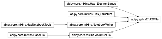
class abipy.eph.a2f.A2fFile(filepath)[source]¶

Bases: abipy.core.mixins.AbinitNcFile, abipy.core.mixins.Has_Structure, abipy.core.mixins.Has_ElectronBands, abipy.core.mixins.NotebookWriter

This file contains the phonon linewidths, EliashbergFunction, the abipy.dfpt.phonons.PhononBands, the abipy.electrons.ebands.ElectronBands and abipy.electrons.ebands.ElectronDos on the k-mesh. Provides methods to analyze and plot results.

Usage example:

with A2fFile("out_A2F.nc") as ncfile:
    print(ncfile)
    ncfile.ebands.plot()
    ncfile.phbands.plot()

Inheritance Diagram

classmethod from_file(filepath)[source]¶: Initialize the object from a netcdf file.

to_string(verbose=0)[source]¶: String representation.

ebands()[source]¶: abipy.electrons.ebands.ElectronBands object.

edos()[source]¶: abipy.electrons.ebands.ElectronDos object with e-DOS computed by Abinit.

property structure¶: abipy.core.structure.Structure object.

property phbands¶: abipy.dfpt.phonons.PhononBands object with frequencies along the q-path. Contains (interpolated) linewidths.

params()[source]¶: OrderedDict with parameters that might be subject to convergence studies.

a2f_qcoarse()[source]¶: A2f with the Eliashberg function a2F(w) computed on the (coarse) ab-initio q-mesh.

a2f_qintp()[source]¶: A2f with the Eliashberg function a2F(w) computed on the dense q-mesh by Fourier interpolation.

get_a2f_qsamp(qsamp)[source]¶: Return the A2f object associated to q-sampling qsamp.

has_a2ftr()[source]¶: True if the netcdf file contains transport data.

a2ftr_qcoarse()[source]¶: A2ftr with the Eliashberg transport spectral function a2F_tr(w, x, x’) computed on the (coarse) ab-initio q-mesh

a2ftr_qintp()[source]¶: A2ftr with the Eliashberg transport spectral function a2F_tr(w, x, x’) computed on the dense q-mesh by Fourier interpolation.

get_a2ftr_qsamp(qsamp)[source]¶: Return the A2ftr object associated to q-sampling qsamp.

close()[source]¶: Close the file.

plot_eph_strength(what_list=('phbands', 'gamma', 'lambda'), ax_list=None, ylims=None, label=None, fontsize=12, **kwargs)[source]¶

Plot phonon bands with EPH coupling strength lambda(q, nu) and lambda(q, nu) These values have been Fourier interpolated by Abinit.

Parameters

what_list – phfreqs for phonons, lambda` for the eph coupling strength, gamma for phonon linewidths.
ax_list – List of matplotlib.axes.Axes (same length as what_list) or None if a new figure should be created.
ylims – Set the data limits for the y-axis. Accept tuple e.g. (left, right) or scalar e.g. left. If left (right) is None, default values are used
label – String used to label the plot in the legend.
fontsize – Legend and title fontsize.

Returns: matplotlib.figure.Figure

Keyword arguments controlling the display of the figure:

kwargs	Meaning
title	Title of the plot (Default: None).
show	True to show the figure (default: True).
savefig	“abc.png” or “abc.eps” to save the figure to a file.
size_kwargs	Dictionary with options passed to fig.set_size_inches e.g. size_kwargs=dict(w=3, h=4)
tight_layout	True to call fig.tight_layout (default: False)
ax_grid	True (False) to add (remove) grid from all axes in fig. Default: None i.e. fig is left unchanged.
ax_annotate	Add labels to subplots e.g. (a), (b). Default: False
fig_close	Close figure. Default: False.

plot(what='gamma', units='eV', scale=None, alpha=0.6, ylims=None, ax=None, colormap='jet', **kwargs)[source]¶

Plot phonon bands with gamma(q, nu) or lambda(q, nu) depending on the vaue of what.

Parameters

what – lambda for eph coupling strength, gamma for phonon linewidths.
units – Units for phonon plots. Possible values in (“eV”, “meV”, “Ha”, “cm-1”, “Thz”). Case-insensitive.
scale – float used to scale the marker size.
alpha – The alpha blending value for the markers between 0 (transparent) and 1 (opaque)
ylims – Set the data limits for the y-axis. Accept tuple e.g. (left, right) or scalar e.g. left. If left (right) is None, default values are used
ax – matplotlib.axes.Axes or None if a new figure should be created.
colormap – matplotlib color map.

Returns: matplotlib.figure.Figure

Keyword arguments controlling the display of the figure:

kwargs	Meaning
title	Title of the plot (Default: None).
show	True to show the figure (default: True).
savefig	“abc.png” or “abc.eps” to save the figure to a file.
size_kwargs	Dictionary with options passed to fig.set_size_inches e.g. size_kwargs=dict(w=3, h=4)
tight_layout	True to call fig.tight_layout (default: False)
ax_grid	True (False) to add (remove) grid from all axes in fig. Default: None i.e. fig is left unchanged.
ax_annotate	Add labels to subplots e.g. (a), (b). Default: False
fig_close	Close figure. Default: False.

plot_a2f_interpol(units='eV', ylims=None, fontsize=8, **kwargs)[source]¶

Compare ab-initio a2F(w) with interpolated values.

Parameters

units – Units for phonon plots. Possible values in (“eV”, “meV”, “Ha”, “cm-1”, “Thz”). Case-insensitive.
ylims – Set the data limits for the y-axis. Accept tuple e.g. (left, right) or scalar e.g. left. If left (right) is None, default values are used
fontsize – Legend and title fontsize

Returns: matplotlib.figure.Figure

Keyword arguments controlling the display of the figure:

kwargs	Meaning
title	Title of the plot (Default: None).
show	True to show the figure (default: True).
savefig	“abc.png” or “abc.eps” to save the figure to a file.
size_kwargs	Dictionary with options passed to fig.set_size_inches e.g. size_kwargs=dict(w=3, h=4)
tight_layout	True to call fig.tight_layout (default: False)
ax_grid	True (False) to add (remove) grid from all axes in fig. Default: None i.e. fig is left unchanged.
ax_annotate	Add labels to subplots e.g. (a), (b). Default: False
fig_close	Close figure. Default: False.

plot_with_a2f(what='gamma', units='eV', qsamp='qintp', phdos=None, ylims=None, **kwargs)[source]¶

Plot phonon bands with lambda(q, nu) + a2F(w) + phonon DOS.

Parameters

what – lambda for eph coupling strength, gamma for phonon linewidths.
units – Units for phonon plots. Possible values in (“eV”, “meV”, “Ha”, “cm-1”, “Thz”). Case-insensitive.
qsamp –
phdos – abipy.dfpt.phonons.PhononDos object. Used to plot the PhononDos on the right.
ylims – Set the data limits for the y-axis. Accept tuple e.g. (left, right) or scalar e.g. left. If left (right) is None, default values are used

Returns: matplotlib.figure.Figure

Keyword arguments controlling the display of the figure:

kwargs	Meaning
title	Title of the plot (Default: None).
show	True to show the figure (default: True).
savefig	“abc.png” or “abc.eps” to save the figure to a file.
size_kwargs	Dictionary with options passed to fig.set_size_inches e.g. size_kwargs=dict(w=3, h=4)
tight_layout	True to call fig.tight_layout (default: False)
ax_grid	True (False) to add (remove) grid from all axes in fig. Default: None i.e. fig is left unchanged.
ax_annotate	Add labels to subplots e.g. (a), (b). Default: False
fig_close	Close figure. Default: False.

yield_figs(**kwargs)[source]¶: This function generates a predefined list of matplotlib figures with minimal input from the user. Used in abiview.py to get a quick look at the results.

write_notebook(nbpath=None)[source]¶: Write a jupyter notebook to nbpath. If nbpath is None, a temporay file in the current working directory is created. Return path to the notebook.

class abipy.eph.a2f.A2fRobot(*args)[source]¶

Bases: abipy.abio.robots.Robot, abipy.electrons.ebands.RobotWithEbands, abipy.dfpt.phonons.RobotWithPhbands

This robot analyzes the results contained in multiple A2F.nc files.

Inheritance Diagram

EXT = 'A2F'¶

linestyle_qsamp = {'qcoarse': '--', 'qintp': '-'}¶

marker_qsamp = {'qcoarse': '^', 'qintp': 'o'}¶

all_qsamps = ['qcoarse']¶

get_dataframe(abspath=False, with_geo=False, with_params=True, funcs=None)[source]¶

Build and return a pandas.DataFrame with the most important results.

Parameters

abspath – True if paths in index should be absolute. Default: Relative to getcwd().
with_geo – True if structure info should be added to the dataframe
funcs – Function or list of functions to execute to add more data to the DataFrame. Each function receives a A2fFile object and returns a tuple (key, value) where key is a string with the name of column and value is the value to be inserted.
with_params – False to exclude calculation parameters from the dataframe.

Return: pandas.DataFrame

plot_lambda_convergence(what='lambda', sortby=None, hue=None, ylims=None, fontsize=8, colormap='jet', **kwargs)[source]¶

Plot the convergence of the lambda(q, nu) parameters wrt to the sortby parameter.

Parameters

what – “lambda” for eph strength, gamma for phonon linewidths.
sortby – Define the convergence parameter, sort files and produce plot labels. Can be None, string or function. If None, no sorting is performed. If string and not empty it’s assumed that the abifile has an attribute with the same name and getattr is invoked. If callable, the output of sortby(abifile) is used.
hue – Variable that define subsets of the data, which will be drawn on separate lines. Accepts callable or string If string, it’s assumed that the abifile has an attribute with the same name and getattr is invoked. If callable, the output of hue(abifile) is used.
ylims – Set the data limits for the y-axis. Accept tuple e.g. (left, right) or scalar e.g. left. If left (right) is None, default values are used
fontsize – Legend and title fontsize.
colormap – matplotlib color map.

Returns: matplotlib.figure.Figure

Keyword arguments controlling the display of the figure:

kwargs	Meaning
title	Title of the plot (Default: None).
show	True to show the figure (default: True).
savefig	“abc.png” or “abc.eps” to save the figure to a file.
size_kwargs	Dictionary with options passed to fig.set_size_inches e.g. size_kwargs=dict(w=3, h=4)
tight_layout	True to call fig.tight_layout (default: False)
ax_grid	True (False) to add (remove) grid from all axes in fig. Default: None i.e. fig is left unchanged.
ax_annotate	Add labels to subplots e.g. (a), (b). Default: False
fig_close	Close figure. Default: False.

plot_a2f_convergence(sortby=None, hue=None, qsamps='all', xlims=None, fontsize=8, colormap='jet', **kwargs)[source]¶

Plot the convergence of the Eliashberg function wrt to the sortby parameter.

Parameters

sortby – Define the convergence parameter, sort files and produce plot labels. Can be None, string or function. If None, no sorting is performed. If string and not empty it’s assumed that the abifile has an attribute with the same name and getattr is invoked. If callable, the output of sortby(abifile) is used.
hue – Variable that define subsets of the data, which will be drawn on separate lines. Accepts callable or string If string, it’s assumed that the abifile has an attribute with the same name and getattr is invoked. If callable, the output of hue(abifile) is used.
qsamps –
xlims – Set the data limits for the x-axis. Accept tuple e.g. (left, right) or scalar e.g. left. If left (right) is None, default values are used.
fontsize – Legend and title fontsize.
colormap – matplotlib color map.

Returns: matplotlib.figure.Figure

Keyword arguments controlling the display of the figure:

kwargs	Meaning
title	Title of the plot (Default: None).
show	True to show the figure (default: True).
savefig	“abc.png” or “abc.eps” to save the figure to a file.
size_kwargs	Dictionary with options passed to fig.set_size_inches e.g. size_kwargs=dict(w=3, h=4)
tight_layout	True to call fig.tight_layout (default: False)
ax_grid	True (False) to add (remove) grid from all axes in fig. Default: None i.e. fig is left unchanged.
ax_annotate	Add labels to subplots e.g. (a), (b). Default: False
fig_close	Close figure. Default: False.

plot_a2fdata_convergence(sortby=None, hue=None, qsamps='all', what_list=('lambda_iso', 'omega_log'), fontsize=8, **kwargs)[source]¶

Plot the convergence of the isotropic lambda and omega_log wrt the sortby parameter.

Parameters

sortby – Define the convergence parameter, sort files and produce plot labels. Can be None, string or function. If None, no sorting is performed. If string and not empty it’s assumed that the abifile has an attribute with the same name and getattr is invoked. If callable, the output of sortby(abifile) is used.
hue – Variable that define subsets of the data, which will be drawn on separate lines. Accepts callable or string If string, it’s assumed that the abifile has an attribute with the same name and getattr is invoked. If callable, the output of hue(abifile) is used.
qsamps –
what_list –
fontsize – Legend and title fontsize.

Returns: matplotlib.figure.Figure

Keyword arguments controlling the display of the figure:

kwargs	Meaning
title	Title of the plot (Default: None).
show	True to show the figure (default: True).
savefig	“abc.png” or “abc.eps” to save the figure to a file.
size_kwargs	Dictionary with options passed to fig.set_size_inches e.g. size_kwargs=dict(w=3, h=4)
tight_layout	True to call fig.tight_layout (default: False)
ax_grid	True (False) to add (remove) grid from all axes in fig. Default: None i.e. fig is left unchanged.
ax_annotate	Add labels to subplots e.g. (a), (b). Default: False
fig_close	Close figure. Default: False.

gridplot_a2f(xlims=None, fontsize=8, sharex=True, sharey=True, **kwargs)[source]¶

Plot grid with a2F(w) and lambda(w) for all files treated by the robot.

Parameters

xlims – Set the data limits for the y-axis. Accept tuple e.g. (left, right) or scalar e.g. left. If left (right) is None, default values are used
sharex – True to share x- and y-axis.
sharey – True to share x- and y-axis.
fontsize – Legend and title fontsize

Keyword arguments controlling the display of the figure:

kwargs	Meaning
title	Title of the plot (Default: None).
show	True to show the figure (default: True).
savefig	“abc.png” or “abc.eps” to save the figure to a file.
size_kwargs	Dictionary with options passed to fig.set_size_inches e.g. size_kwargs=dict(w=3, h=4)
tight_layout	True to call fig.tight_layout (default: False)
ax_grid	True (False) to add (remove) grid from all axes in fig. Default: None i.e. fig is left unchanged.
ax_annotate	Add labels to subplots e.g. (a), (b). Default: False
fig_close	Close figure. Default: False.

yield_figs(**kwargs)[source]¶: This function generates a predefined list of matplotlib figures with minimal input from the user.

write_notebook(nbpath=None)[source]¶: Write a jupyter notebook to nbpath. If nbpath is None, a temporay file in the current working directory is created. Return path to the notebook.

class abipy.eph.a2f.A2fReader(path)[source]¶

Bases: abipy.eph.common.BaseEphReader

Reads data from the EPH.nc file and constructs objects.

Inheritance Diagram

read_edos()[source]¶: Read the abipy.electrons.ebands.ElectronDos used to compute EPH quantities.

read_phbands_qpath()[source]¶: Read and return a abipy.dfpt.phonons.PhononBands object with frequencies computed along the q-path.

read_phlambda_qpath(sum_spin=True)[source]¶

Reads the EPH coupling strength interpolated along the q-path.

Returns: numpy.ndarray with shape [nqpath, natom3] if not sum_spin else [nsppol, nqpath, natom3]

read_phgamma_qpath(sum_spin=True)[source]¶

Reads the phonon linewidths (eV) interpolated along the q-path.

Returns: numpy.ndarray with shape [nqpath, natom3] if not sum_spin else [nsppol, nqpath, natom3]

read_a2f(qsamp)[source]¶: Read and return the Eliashberg function A2F.

`common` Module ¶

Objects common to the other eph modules.

class abipy.eph.common.BaseEphReader(path)[source]¶

Bases: abipy.electrons.ebands.ElectronsReader

Provides methods common to the netcdf files produced by the EPH code. See Abinit docs for the meaning of the variables.

ddb_ngqpt()[source]¶: Q-Mesh for DDB file.

ngqpt()[source]¶: Effective Q-mesh used in to compute integrals (ph_linewidts, e-ph self-energy).

ph_ngqpt()[source]¶: Q-mesh for Phonon DOS, interpolated A2F …

eph_ngqpt_fine()[source]¶: Q-mesh for interpolated DFPT potentials

common_eph_params()[source]¶: Read basic parameters (scalars) from the netcdf files produced by the EPH code and cache them

abipy.eph.common.glr_frohlich(qpoint, becs_cart, epsinf_cart, phdispl_cart_bohr, phfreqs_ha, structure, qdamp=None, eph_wtol=1e-06, tol_qnorm=1e-06)[source]¶

Compute the long-range part of the e-ph matrix element with the simplified Frohlich model i.e. we include only G = 0 and the <k+q,b1|e^{i(q+G).r}|b2,k> coefficient is replaced by delta_{b1, b2}

Parameters

qpoint – abipy.core.kpoints.Kpoint object.
becs_cart – (natom, 3, 3) arrays with Born effective charges in Cartesian coordinates.
epsinf_cart – (3, 3) array with macroscopic dielectric tensor in Cartesian coordinates.
phdispl_cart_bohr – (natom3_nu, natom3) complex array with phonon displacement in Cartesian coordinates (Bohr)
phfreqs_ha – (3 * natom) array with phonon frequencies in Ha.
structure – abipy.core.structure.Structure object.
qdamp – Exponential damping.
eph_wtol – Set g to zero below this phonon frequency.
tol_qnorm – Tolerance of the norm of the q-point.

Returns

(natom3) complex array with glr_nu.

`eph_plotter` Module ¶

Objects to plot electronic, vibrational and e-ph properties.

class abipy.eph.eph_plotter.EphPlotter(ebands_kpath, phbst_file, phdos_file, ebands_kmesh=None)[source]¶

Bases: object

This object provides methods to plot electron and phonons for a single system. An EphPlotter has:

An abipy.electrons.ebands.ElectronBands on a k-path

An abipy.electrons.ebands.ElectronBands on a k-mesh (optional)

A abipy.dfpt.phonons.PhbstFile with phonons along a q-path.

A abipy.dfpt.phonons.PhdosFile with different kinds of phonon DOSes.

EphPlotter uses these objects/files and other inputs/files provided by the user to generate matplotlib plots related to e-ph interaction.

Inheritance Diagram

classmethod from_ddb(ddb, ebands_kpath, ebands_kmesh=None, **kwargs)[source]¶

Build the object from the ddb file, invoke anaddb to get phonon properties. This entry point is needed to have phonon plots with LO-TO splitting as AbiPy will generate an anaddb input with the different q –> 0 directions required in phbands.plot to plot the LO-TO splitting correctly.

Parameters

ddb – abipy.dfpt.ddb.DdbFile or filepath.
ebands_kpath – abipy.electrons.ebands.ElectronBands with energies on a k-path or filepath.
ebands_kpath – (optional) abipy.electrons.ebands.ElectronBands with energies on a k-mesh or filepath.
kwargs – Passed to anaget_phbst_and_phdos_files

plot(eb_ylims=None, **kwargs)[source]¶

Plot electrons with possible (phonon-mediated) scattering channels for the CBM and VBM. Also plot phonon band structure and phonon PJDOS.

Parameters: eb_ylims – Set the data limits for the y-axis of the electron band. Accept tuple e.g. (left, right) or scalar e.g. left. If None, limits are selected automatically.

Return: matplotlib.figure.Figure

Keyword arguments controlling the display of the figure:

kwargs	Meaning
title	Title of the plot (Default: None).
show	True to show the figure (default: True).
savefig	“abc.png” or “abc.eps” to save the figure to a file.
size_kwargs	Dictionary with options passed to fig.set_size_inches e.g. size_kwargs=dict(w=3, h=4)
tight_layout	True to call fig.tight_layout (default: False)
ax_grid	True (False) to add (remove) grid from all axes in fig. Default: None i.e. fig is left unchanged.
ax_annotate	Add labels to subplots e.g. (a), (b). Default: False
fig_close	Close figure. Default: False.

plot_phonons_occ(temps=(100, 200, 300, 400), **kwargs)[source]¶

Plot phonon band structure with markers proportional to the occupation of each phonon mode for different temperatures.

Parameters: temps – List of temperatures in Kelvin.

Return: matplotlib.figure.Figure

Keyword arguments controlling the display of the figure:

kwargs	Meaning
title	Title of the plot (Default: None).
show	True to show the figure (default: True).
savefig	“abc.png” or “abc.eps” to save the figure to a file.
size_kwargs	Dictionary with options passed to fig.set_size_inches e.g. size_kwargs=dict(w=3, h=4)
tight_layout	True to call fig.tight_layout (default: False)
ax_grid	True (False) to add (remove) grid from all axes in fig. Default: None i.e. fig is left unchanged.
ax_annotate	Add labels to subplots e.g. (a), (b). Default: False
fig_close	Close figure. Default: False.

plot_linewidths_sigeph(sigeph, eb_ylims=None, **kwargs)[source]¶

Plot e-bands + e-DOS + Im(Sigma_{eph}) + phonons + gkq^2

Parameters

sigeph – abipy.electrons.eph.SigephFile or string with path to file.
eb_ylims – Set the data limits for the y-axis of the electron band. Accept tuple e.g. (left, right) or scalar e.g. left. If None, limits are selected automatically.

Keyword arguments controlling the display of the figure:

kwargs	Meaning
title	Title of the plot (Default: None).
show	True to show the figure (default: True).
savefig	“abc.png” or “abc.eps” to save the figure to a file.
size_kwargs	Dictionary with options passed to fig.set_size_inches e.g. size_kwargs=dict(w=3, h=4)
tight_layout	True to call fig.tight_layout (default: False)
ax_grid	True (False) to add (remove) grid from all axes in fig. Default: None i.e. fig is left unchanged.
ax_annotate	Add labels to subplots e.g. (a), (b). Default: False
fig_close	Close figure. Default: False.

`rta` Module ¶

RTA.nc file.

class abipy.eph.rta.RtaFile(filepath)[source]¶

Bases: abipy.core.mixins.AbinitNcFile, abipy.core.mixins.Has_Structure, abipy.core.mixins.Has_ElectronBands, abipy.core.mixins.NotebookWriter

classmethod from_file(filepath)[source]¶: Initialize the object from a netcdf file.

property ntemp¶: Number of temperatures.

property tmesh¶: Mesh with Temperatures in Kelvin.

assume_gap()[source]¶: True if we are dealing with a semiconductor. More precisely if all(sigma_erange) > 0.

has_ibte()[source]¶: True if file contains IBTE results.

ebands()[source]¶: abipy.electrons.ebands.ElectronBands object.

property structure¶: abipy.core.structure.Structure object.

params()[source]¶: OrderedDict with parameters that might be subject to convergence studies.

to_string(verbose=0)[source]¶: String representation.

get_mobility_mu(eh, itemp, component='xx', ef=None, irta=0, spin=0)[source]¶

Get the mobility at the chemical potential Ef

Parameters

eh – 0 for electrons, 1 for holes.
itemp – Index of the temperature.
component – Cartesian component to plot: “xx”, “yy” “xy” …
ef – Value of the doping in eV. The default None uses the chemical potential at the temperature item as computed by Abinit.
spin – Spin index.

plot_edos(ax=None, fontsize=8, **kwargs)[source]¶

Plot electron DOS

Parameters

ax – matplotlib.axes.Axes or None if a new figure should be created.
fontsize (int) – fontsize for titles and legend

Return: matplotlib.figure.Figure

Keyword arguments controlling the display of the figure:

kwargs	Meaning
title	Title of the plot (Default: None).
show	True to show the figure (default: True).
savefig	“abc.png” or “abc.eps” to save the figure to a file.
size_kwargs	Dictionary with options passed to fig.set_size_inches e.g. size_kwargs=dict(w=3, h=4)
tight_layout	True to call fig.tight_layout (default: False)
ax_grid	True (False) to add (remove) grid from all axes in fig. Default: None i.e. fig is left unchanged.
ax_annotate	Add labels to subplots e.g. (a), (b). Default: False
fig_close	Close figure. Default: False.

plot_tau_isoe(ax_list=None, colormap='jet', fontsize=8, **kwargs)[source]¶

Plot tau(e). Energy-dependent scattering rate defined by:

$tau(epsilon) = frac{1}{N_k} sum_{nk} tau_{nk},delta(epsilon - epsilon_{nk})$

Two differet subplots for SERTA and MRTA.

Parameters

ax_list – List of matplotlib.axes.Axes or None if a new figure should be created.
colormap –
fontsize (int) – fontsize for titles and legend

Return: matplotlib.figure.Figure

Keyword arguments controlling the display of the figure:

kwargs	Meaning
title	Title of the plot (Default: None).
show	True to show the figure (default: True).
savefig	“abc.png” or “abc.eps” to save the figure to a file.
size_kwargs	Dictionary with options passed to fig.set_size_inches e.g. size_kwargs=dict(w=3, h=4)
tight_layout	True to call fig.tight_layout (default: False)
ax_grid	True (False) to add (remove) grid from all axes in fig. Default: None i.e. fig is left unchanged.
ax_annotate	Add labels to subplots e.g. (a), (b). Default: False
fig_close	Close figure. Default: False.

plot_vvtau_dos(component='xx', spin=0, ax=None, colormap='jet', fontsize=8, **kwargs)[source]¶

Plot (v_i * v_j * tau) DOS.

$frac{1}{N_k} sum_{nk} v_i v_j delta(epsilon - epsilon_{nk})$

Parameters

component – Cartesian component to plot: “xx”, “yy” “xy” …
ax – matplotlib.axes.Axes or None if a new figure should be created.
colormap – matplotlib colormap.
fontsize (int) – fontsize for titles and legend

Return: matplotlib.figure.Figure

Keyword arguments controlling the display of the figure:

kwargs	Meaning
title	Title of the plot (Default: None).
show	True to show the figure (default: True).
savefig	“abc.png” or “abc.eps” to save the figure to a file.
size_kwargs	Dictionary with options passed to fig.set_size_inches e.g. size_kwargs=dict(w=3, h=4)
tight_layout	True to call fig.tight_layout (default: False)
ax_grid	True (False) to add (remove) grid from all axes in fig. Default: None i.e. fig is left unchanged.
ax_annotate	Add labels to subplots e.g. (a), (b). Default: False
fig_close	Close figure. Default: False.

plot_mobility(eh=0, irta=0, component='xx', spin=0, ax=None, colormap='jet', fontsize=8, yscale='log', **kwargs)[source]¶

Read the mobility from the netcdf file and plot it

Parameters

component – Component to plot: “xx”, “yy” “xy” …
ax – matplotlib.axes.Axes or None if a new figure should be created.
colormap – matplotlib colormap.
fontsize (int) – fontsize for titles and legend

Return: matplotlib.figure.Figure

Keyword arguments controlling the display of the figure:

kwargs	Meaning
title	Title of the plot (Default: None).
show	True to show the figure (default: True).
savefig	“abc.png” or “abc.eps” to save the figure to a file.
size_kwargs	Dictionary with options passed to fig.set_size_inches e.g. size_kwargs=dict(w=3, h=4)
tight_layout	True to call fig.tight_layout (default: False)
ax_grid	True (False) to add (remove) grid from all axes in fig. Default: None i.e. fig is left unchanged.
ax_annotate	Add labels to subplots e.g. (a), (b). Default: False
fig_close	Close figure. Default: False.

plot_transport_tensors_mu(component='xx', spin=0, what_list=('sigma', 'seebeck', 'kappa', 'pi'), colormap='jet', fontsize=8, **kwargs)[source]¶

Plot selected Cartesian components of transport tensors as a function of the chemical potential mu at the given temperature.

Parameters

ax_list – matplotlib.axes.Axes or None if a new figure should be created.
fontsize – fontsize for legends and titles

Return: matplotlib.figure.Figure

Keyword arguments controlling the display of the figure:

kwargs	Meaning
title	Title of the plot (Default: None).
show	True to show the figure (default: True).
savefig	“abc.png” or “abc.eps” to save the figure to a file.
size_kwargs	Dictionary with options passed to fig.set_size_inches e.g. size_kwargs=dict(w=3, h=4)
tight_layout	True to call fig.tight_layout (default: False)
ax_grid	True (False) to add (remove) grid from all axes in fig. Default: None i.e. fig is left unchanged.
ax_annotate	Add labels to subplots e.g. (a), (b). Default: False
fig_close	Close figure. Default: False.

plot_ibte_vs_rta_rho(component='xx', fontsize=8, ax=None, **kwargs)[source]¶

Plot resistivity computed with SERTA, MRTA and IBTE

Keyword arguments controlling the display of the figure:

kwargs	Meaning
title	Title of the plot (Default: None).
show	True to show the figure (default: True).
savefig	“abc.png” or “abc.eps” to save the figure to a file.
size_kwargs	Dictionary with options passed to fig.set_size_inches e.g. size_kwargs=dict(w=3, h=4)
tight_layout	True to call fig.tight_layout (default: False)
ax_grid	True (False) to add (remove) grid from all axes in fig. Default: None i.e. fig is left unchanged.
ax_annotate	Add labels to subplots e.g. (a), (b). Default: False
fig_close	Close figure. Default: False.

yield_figs(**kwargs)[source]¶: Return figures plotting the transport data

close()[source]¶: Close the file.

write_notebook(nbpath=None)[source]¶: Write a jupyter notebook to nbpath. If nbpath is None, a temporay file in the current working directory is created. Return path to the notebook.

class abipy.eph.rta.RtaRobot(*args)[source]¶

Bases: abipy.abio.robots.Robot, abipy.electrons.ebands.RobotWithEbands

This robot analyzes the results contained in multiple RTA.nc files.

Inheritance Diagram

EXT = 'RTA'¶

plot_mobility_kconv(eh=0, bte=('serta', 'mrta', 'ibte'), component='xx', itemp=0, spin=0, fontsize=14, ax=None, **kwargs)[source]¶

Plot the convergence of the mobility as a function of the number of k-points, for different transport formalisms included in the computation.

Parameters

eh – 0 for electrons, 1 for holes.
bte – list of transport formalism to plot (serta, mrta, ibte)
component – Cartesian component to plot (‘xx’, ‘xy’, …)
itemp – temperature index.
spin – Spin index.
fontsize – fontsize for legends and titles
ax – matplotlib.axes.Axes or None if a new figure should be created.

Returns: matplotlib.figure.Figure

Keyword arguments controlling the display of the figure:

kwargs	Meaning
title	Title of the plot (Default: None).
show	True to show the figure (default: True).
savefig	“abc.png” or “abc.eps” to save the figure to a file.
size_kwargs	Dictionary with options passed to fig.set_size_inches e.g. size_kwargs=dict(w=3, h=4)
tight_layout	True to call fig.tight_layout (default: False)
ax_grid	True (False) to add (remove) grid from all axes in fig. Default: None i.e. fig is left unchanged.
ax_annotate	Add labels to subplots e.g. (a), (b). Default: False
fig_close	Close figure. Default: False.

assume_gap()[source]¶: True if we are dealing with a semiconductor. More precisely if all(sigma_erange) > 0.

all_have_ibte()[source]¶: True if all files contain IBTE results.

get_same_tmesh()[source]¶: Check whether all files have the same T-mesh. Return common tmesh else raise RuntimeError.

plot_ibte_vs_rta_rho(component='xx', fontsize=8, **kwargs)[source]¶

plot_ibte_mrta_serta_conv(what='resistivity', fontsize=8, **kwargs)[source]¶

yield_figs(**kwargs)[source]¶: This function generates a predefined list of matplotlib figures with minimal input from the user. Used in abiview.py to get a quick look at the results.

write_notebook(nbpath=None)[source]¶: Write a jupyter notebook to nbpath. If nbpath is None, a temporay file in the current working directory is created. Return path to the notebook.

`sigeph` Module ¶

This module contains objects for postprocessing e-ph calculations using the results stored in the SIGEPH.nc file.

For a theoretical introduction see [Giustino2017]

class abipy.eph.sigeph.QpTempState(spin, kpoint, band, tmesh, e0, qpe, ze0, fan0, dw, qpe_oms)[source]¶

Bases: abipy.eph.sigeph.QpTempState

Quasi-particle result for given (spin, kpoint, band).

Note

Energies are in eV.

qpeme0()[source]¶: E_QP[T] - E_0 (Real part)

re_qpe()[source]¶: Real part of the QP energy.

imag_qpe()[source]¶: Imaginay part of the QP energy.

property re_fan0¶: Real part of the Fan term at KS.

property imag_fan0¶: Imaginary part of the Fan term at KS.

re_sig0()[source]¶: Real part of the self-energy computed at the KS energy.

imag_sig0()[source]¶: Imaginary part of the self-energy computed at the KS energy.

skb()[source]¶: Tuple with (spin, kpoint, band)

classmethod get_fields(exclude=())[source]¶

to_string(verbose=0, title=None)[source]¶: String representation with verbosity level verbose and optional title.

get_dataframe(index=None, with_spin=True, params=None)[source]¶

Build pandas dataframe with QP results

Parameters

index – dataframe index.
with_spin – False if spin index is not wanted.
params – Optional (Ordered) dictionary with extra parameters.

Return: pandas.DataFrame

classmethod get_fields_for_plot(vs, with_fields, exclude_fields)[source]¶

Return list of QpTempState fields to plot from input arguments.

Parameters

in ["temp" (vs) –
"e0"] –
with_fields –
exclude_fields –

plot(with_fields='all', exclude_fields=None, ax_list=None, label=None, fontsize=12, **kwargs)[source]¶

Plot the QP results as function of temperature.

Parameters

with_fields – The names of the QpTempState attributes to plot as function of e0. Accepts: List of strings or string with tokens separated by blanks. See QpTempState for the list of available fields.
exclude_fields – Similar to with_field but excludes fields.
ax_list – List of matplotlib axes for plot. If None, new figure is produced.
label – Label for plot.
fontsize – Fontsize for legend and title.

Returns: matplotlib.figure.Figure

Keyword arguments controlling the display of the figure:

kwargs	Meaning
title	Title of the plot (Default: None).
show	True to show the figure (default: True).
savefig	“abc.png” or “abc.eps” to save the figure to a file.
size_kwargs	Dictionary with options passed to fig.set_size_inches e.g. size_kwargs=dict(w=3, h=4)
tight_layout	True to call fig.tight_layout (default: False)
ax_grid	True (False) to add (remove) grid from all axes in fig. Default: None i.e. fig is left unchanged.
ax_annotate	Add labels to subplots e.g. (a), (b). Default: False
fig_close	Close figure. Default: False.

class abipy.eph.sigeph.QpTempList(*args, **kwargs)[source]¶

Bases: list

A list of quasiparticle corrections (usually for a given spin).

property tmesh¶: Temperature mesh in Kelvin.

property ntemp¶: Number of temperatures.

to_string(verbose=0, title=None)[source]¶: String representation.

sort_by_e0()[source]¶: Return a new QpTempList object with the E0 energies sorted in ascending order.

get_e0mesh()[source]¶: Return the E0 energies.

get_field_itemp(field, itemp)[source]¶: numpy.ndarray containing the values of field at temperature itemp

merge(other, copy=False)[source]¶

Merge self with other. Return new QpTempList object

Raise: ValueError if merge cannot be done.

plot_vs_e0(itemp_list=None, with_fields='all', reim='real', function=<function QpTempList.<lambda>>, exclude_fields=None, fermie=None, colormap='jet', ax_list=None, xlims=None, ylims=None, exchange_xy=False, fontsize=12, **kwargs)[source]¶

Plot QP results as a function of the initial KS energy.

Parameters

itemp_list – List of integers to select a particular temperature. None for all
with_fields – The names of the QP attributes to plot as function of e0. Accepts: List of strings or string with tokens separated by blanks. See QPState for the list of available fields.
reim – Plot the real or imaginary part
function – Apply a function to the results before plotting
exclude_fields – Similar to with_field but excludes fields.
fermie – Value of the Fermi level used in plot. None for absolute e0s.
colormap – matplotlib color map.
ax_list – List of matplotlib.axes.Axes for plot. If None, new figure is produced.
xlims – Set the data limits for the x-axis. Accept tuple e.g. (left, right) or scalar e.g. left. If left (right) is None, default values are used.
ylims – Set the data limits for the x-axis. Accept tuple e.g. (left, right) or scalar e.g. left. If left (right) is None, default values are used.
exchange_xy – True to exchange x-y axis.
fontsize – Legend and title fontsize.
kwargs – linestyle, color, label, marker

Returns: matplotlib.figure.Figure

Keyword arguments controlling the display of the figure:

kwargs	Meaning
title	Title of the plot (Default: None).
show	True to show the figure (default: True).
savefig	“abc.png” or “abc.eps” to save the figure to a file.
size_kwargs	Dictionary with options passed to fig.set_size_inches e.g. size_kwargs=dict(w=3, h=4)
tight_layout	True to call fig.tight_layout (default: False)
ax_grid	True (False) to add (remove) grid from all axes in fig. Default: None i.e. fig is left unchanged.
ax_annotate	Add labels to subplots e.g. (a), (b). Default: False
fig_close	Close figure. Default: False.

class abipy.eph.sigeph.EphSelfEnergy(wmesh, qp, vals_e0ks, dvals_de0ks, dw_vals, vals_wr, spfunc_wr, frohl_vals_e0ks=None, frohl_dvals_de0ks=None, frohl_spfunc_wr=None)[source]¶

Bases: object

Electron self-energy due to phonon interaction $\Sigma_{nk}(\omega,T)$ Actually this object stores the diagonal matrix elements in the KS basis set.

latex_symbol = {'im': '$\\Im{\\Sigma(\\omega)}$', 're': '$\\Re{\\Sigma(\\omega)}$', 'spfunc': '$A(\\omega)}$'}¶

to_string(verbose=0, title=None)[source]¶: String representation.

plot_tdep(itemps='all', zero_energy='e0', colormap='jet', ax_list=None, what_list=('re', 'im', 'spfunc'), with_frohl=False, xlims=None, fontsize=8, **kwargs)[source]¶

Plot the real/imaginary part of self-energy as well as the spectral function for the different temperatures with a colormap.

Parameters

itemps – List of temperature indices. “all” to plot’em all.
zero_energy –
colormap – matplotlib color map.
ax_list – List of matplotlib.axes.Axes. If None, new figure is produced.
what_list – List of strings selecting the quantity to plot. “re” for real part, “im” for imaginary part, “spfunc” for spectral function A(omega).
with_frohl – Visualize Frohlich contribution (if present).
xlims – Set the data limits for the x-axis. Accept tuple e.g. (left, right) or scalar e.g. left. If left (right) is None, default values are used.
fontsize – legend and label fontsize.
kwargs – Keyword arguments passed to ax.plot

Returns: matplotlib.figure.Figure

Keyword arguments controlling the display of the figure:

kwargs	Meaning
title	Title of the plot (Default: None).
show	True to show the figure (default: True).
savefig	“abc.png” or “abc.eps” to save the figure to a file.
size_kwargs	Dictionary with options passed to fig.set_size_inches e.g. size_kwargs=dict(w=3, h=4)
tight_layout	True to call fig.tight_layout (default: False)
ax_grid	True (False) to add (remove) grid from all axes in fig. Default: None i.e. fig is left unchanged.
ax_annotate	Add labels to subplots e.g. (a), (b). Default: False
fig_close	Close figure. Default: False.

plot(itemps='all', zero_energy='e0', colormap='jet', ax_list=None, what_list=('re', 'im', 'spfunc'), with_frohl=False, xlims=None, fontsize=8, **kwargs)¶

Plot the real/imaginary part of self-energy as well as the spectral function for the different temperatures with a colormap.

Parameters

itemps – List of temperature indices. “all” to plot’em all.
zero_energy –
colormap – matplotlib color map.
ax_list – List of matplotlib.axes.Axes. If None, new figure is produced.
what_list – List of strings selecting the quantity to plot. “re” for real part, “im” for imaginary part, “spfunc” for spectral function A(omega).
with_frohl – Visualize Frohlich contribution (if present).
xlims – Set the data limits for the x-axis. Accept tuple e.g. (left, right) or scalar e.g. left. If left (right) is None, default values are used.
fontsize – legend and label fontsize.
kwargs – Keyword arguments passed to ax.plot

Returns: matplotlib.figure.Figure

Keyword arguments controlling the display of the figure:

kwargs	Meaning
title	Title of the plot (Default: None).
show	True to show the figure (default: True).
savefig	“abc.png” or “abc.eps” to save the figure to a file.
size_kwargs	Dictionary with options passed to fig.set_size_inches e.g. size_kwargs=dict(w=3, h=4)
tight_layout	True to call fig.tight_layout (default: False)
ax_grid	True (False) to add (remove) grid from all axes in fig. Default: None i.e. fig is left unchanged.
ax_annotate	Add labels to subplots e.g. (a), (b). Default: False
fig_close	Close figure. Default: False.

plot_qpsolution(itemp=0, with_int_aw=True, ax_list=None, xlims=None, fontsize=8, **kwargs)[source]¶

Graphical representation of the QP solution(s) along the real axis including the approximated solution obtained with the linearized equation and the on-the-mass-shell approach.

Produce two subplots:

Re/Imag part and intersection with omega - eKs
A(w) + int^w A(w’)dw’ + OTMS

Parameters

itemp – Temperature index.
ax_list – List of matplotlib.axes.Axes. If None, new figure is produced.
with_int_aw – Plot cumulative integral of A(w).
xlims – Set the data limits for the x-axis. Accept tuple e.g. (left, right) or scalar e.g. left. If left (right) is None, default values are used.
fontsize – legend and label fontsize.
kwargs – Keyword arguments passed to ax.plot

Returns: matplotlib.figure.Figure

Keyword arguments controlling the display of the figure:

kwargs	Meaning
title	Title of the plot (Default: None).
show	True to show the figure (default: True).
savefig	“abc.png” or “abc.eps” to save the figure to a file.
size_kwargs	Dictionary with options passed to fig.set_size_inches e.g. size_kwargs=dict(w=3, h=4)
tight_layout	True to call fig.tight_layout (default: False)
ax_grid	True (False) to add (remove) grid from all axes in fig. Default: None i.e. fig is left unchanged.
ax_annotate	Add labels to subplots e.g. (a), (b). Default: False
fig_close	Close figure. Default: False.

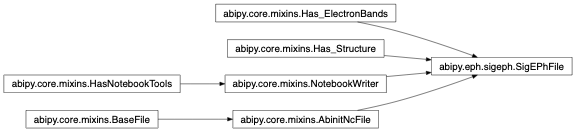
class abipy.eph.sigeph.SigEPhFile(filepath)[source]¶

Bases: abipy.core.mixins.AbinitNcFile, abipy.core.mixins.Has_Structure, abipy.core.mixins.Has_ElectronBands, abipy.core.mixins.NotebookWriter

This file contains the Fan-Migdal Debye-Waller self-energy, the abipy.electrons.ebands.ElectronBands on the k-mesh. Provides methods to analyze and plot results.

Usage example:

with SigEPhFile("out_SIGEPH.nc") as ncfile:
    print(ncfile)
    ncfile.ebands.plot()

Inheritance Diagram

marker_spin = {0: '^', 1: 'v'}¶

color_spin = {0: 'k', 1: 'r'}¶

classmethod from_file(filepath)[source]¶: Initialize the object from a netcdf file.

to_string(verbose=0)[source]¶: String representation.

ebands()[source]¶: abipy.electrons.ebands.ElectronBands object.

property structure¶: abipy.core.structure.Structure object.

close()[source]¶: Close the file.

has_spectral_function()[source]¶: True if file contains spectral function data.

has_eliashberg_function()[source]¶: True if file contains Eliashberg functions.

property sigma_kpoints¶: The K-points where QP corrections have been calculated.

property tmesh¶: Temperature mesh in Kelvin.

kcalc2ibz()[source]¶: Return a mapping of the kpoints at which the self energy was calculated and the ibz i.e. the list of k-points in the band structure used to construct the self-energy.

ibz2kcalc()[source]¶: Mapping IBZ –> K-points in self-energy. Set to -1 if IBZ k-point not present.

ks_dirgaps()[source]¶: numpy.ndarray of shape [nsppol, nkcalc] with the KS gaps in eV ordered as kcalc.

qp_dirgaps_t()[source]¶: numpy.ndarray of shape [nsppol, nkcalc, ntemp] with the QP direct gap in eV ordered as kcalc. QP energies are computed with the linearized QP equation (Z factor)

qp_dirgaps_otms_t()[source]¶: numpy.ndarray of shape [nsppol, nkcalc, ntemp] with the QP direct gap in eV ordered as kcalc. QP energies are computed with the on-the-mass-shell approximation

mu_e()[source]¶: mu_e[ntemp] chemical potential (eV) of electrons for the different temperatures.

edos()[source]¶: abipy.electrons.ebands.ElectronDos object computed by Abinit with the input WFK file without doping (if any). Since this field is optional, None is returned if netcdf variable is not present

sigkpt2index(kpoint)[source]¶: Returns the index of the self-energy k-point in sigma_kpoints Used to access data in the arrays that are dimensioned with [0:nkcalc]

find_qpkinds(qp_kpoints)[source]¶: Find kpoints for QP corrections from user input. Return list of (kpt, ikcalc) tuples where kpt is a abipy.core.kpoints.Kpoint and ikcalc is the index in the nkcalc array..

params()[source]¶: OrderedDict with the convergence parameters, e.g. nbsum.

get_sigeph_skb(spin, kpoint, band)[source]¶: “Return e-ph self-energy for the given (spin, kpoint, band).

get_dataframe(itemp=None, with_params=True, with_spin='auto', ignore_imag=False)[source]¶

Returns pandas.DataFrame with QP results for all k-points, bands and spins included in the calculation.

Parameters

itemp – Temperature index, if None all temperatures are returned.
with_params – False to exclude calculation parameters from the dataframe.
ignore_imag – only real part is returned if ignore_imag.

get_dirgaps_dataframe(kpoint, itemp=None, spin=0, with_params=False)[source]¶

Returns pandas.DataFrame with QP direct gaps at the given k-point

Parameters

kpoint – K-point in self-energy. Accepts abipy.core.kpoints.Kpoint, vector or index.
itemp – Temperature index, if None all temperatures are returned.
spin – Spin index
with_params – False to exclude calculation parameters from the dataframe.

get_dataframe_sk(spin, kpoint, itemp=None, index=None, with_params=False, with_spin='auto', ignore_imag=False)[source]¶

Returns pandas.DataFrame with QP results for the given (spin, k-point).

Parameters

spin – Spin index.
kpoint – K-point in self-energy. Accepts abipy.core.kpoints.Kpoint, vector or index.
itemp – Temperature index, if None all temperatures are returned.
index – dataframe index.
with_params – False to exclude calculation parameters from the dataframe.
with_spin – True to add column with spin index. “auto” to add it only if nsppol == 2
ignore_imag – Only real part is returned if ignore_imag.

get_linewidth_dos(method='gaussian', e0='fermie', step=0.1, width=0.2)[source]¶

Calculate linewidth density of states

Parameters

method – String defining the method for the computation of the DOS.
step – Energy step (eV) of the linear mesh.
width – Standard deviation (eV) of the gaussian.

Returns: abipy.electrons.ebands.ElectronDos object.

get_qp_array(ks_ebands_kpath=None, mode='qp', rta_type='mrta')[source]¶

Get the lifetimes in an array with spin, kpoint and band dimensions

Parameters: rta_type – “serta” for SERTA linewidths or “mrta” for MRTA linewidths.

get_lifetimes_boltztrap(basename, rta_type='mrta', workdir=None)[source]¶

Produce basename.tau and basename.energy text files to be used in Boltztrap code for transport calculations.

Parameters

basename – The basename of the files to be produced
workdir – Directory where files will be produced. None for current working directory.

interpolate(itemp_list=None, lpratio=5, mode='qp', ks_ebands_kpath=None, ks_ebands_kmesh=None, ks_degatol=0.0001, vertices_names=None, line_density=20, filter_params=None, only_corrections=False, verbose=0)[source]¶

Interpolated the self-energy corrections in k-space on a k-path and, optionally, on a k-mesh.

Parameters

itemp_list – List of temperature indices to interpolate. None for all.
lpratio – Ratio between the number of star functions and the number of ab-initio k-points. The default should be OK in many systems, larger values may be required for accurate derivatives.
mode – Interpolation mode, can be ‘qp’ or ‘ks+lifetimes’
ks_ebands_kpath – KS abipy.electrons.ebands.ElectronBands on a k-path. If present, the routine interpolates the QP corrections and apply them on top of the KS band structure This is the recommended option because QP corrections are usually smoother than the QP energies and therefore easier to interpolate. If None, the QP energies are interpolated along the path defined by vertices_names and line_density.
ks_ebands_kmesh – KS abipy.electrons.ebands.ElectronBands on a homogeneous k-mesh. If present, the routine interpolates the corrections on the k-mesh (used to compute the QP DOS)
ks_degatol – Energy tolerance in eV. Used when either ks_ebands_kpath or ks_ebands_kmesh are given. KS energies are assumed to be degenerate if they differ by less than this value. The interpolator may break band degeneracies (the error is usually smaller if QP corrections are interpolated instead of QP energies). This problem can be partly solved by averaging the interpolated values over the set of KS degenerate states. A negative value disables this ad-hoc symmetrization.
vertices_names – Used to specify the k-path for the interpolated QP band structure when ks_ebands_kpath is None. It’s a list of tuple, each tuple is of the form (kfrac_coords, kname) where kfrac_coords are the reduced coordinates of the k-point and kname is a string with the name of the k-point. Each point represents a vertex of the k-path. line_density defines the density of the sampling. If None, the k-path is automatically generated according to the point group of the system.
line_density – Number of points in the smallest segment of the k-path. Used with vertices_names.
filter_params – TO BE DESCRIBED
only_corrections – If True, the output contains the interpolated QP corrections instead of the QP energies. Available only if ks_ebands_kpath and/or ks_ebands_kmesh are used.
verbose – Verbosity level

Returns: class:TdepElectronBands.

plot_qpgaps_t(qp_kpoints=0, qp_type='qpz0', ax_list=None, plot_qpmks=True, fontsize=8, **kwargs)[source]¶

Plot the KS and the QP(T) direct gaps for all the k-points available in the SIGEPH file.

Parameters

qp_kpoints – List of k-points in self-energy. Accept integers (list or scalars), list of vectors, or None to plot all k-points.
qp_type – “qpz0” for linearized QP equation with Z factor at KS e0, “otms” for on-the-mass-shell results.
ax_list – List of matplotlib.axes.Axes or None if a new figure should be created.
plot_qpmks – If False, plot QP_gap, KS_gap else (QP_gap - KS_gap)
fontsize – legend and title fontsize.
kwargs – Passed to ax.plot method except for marker.

Returns: matplotlib.figure.Figure

Keyword arguments controlling the display of the figure:

kwargs	Meaning
title	Title of the plot (Default: None).
show	True to show the figure (default: True).
savefig	“abc.png” or “abc.eps” to save the figure to a file.
size_kwargs	Dictionary with options passed to fig.set_size_inches e.g. size_kwargs=dict(w=3, h=4)
tight_layout	True to call fig.tight_layout (default: False)
ax_grid	True (False) to add (remove) grid from all axes in fig. Default: None i.e. fig is left unchanged.
ax_annotate	Add labels to subplots e.g. (a), (b). Default: False
fig_close	Close figure. Default: False.

plot_qpdata_t(spin, kpoint, band_list=None, fontsize=12, **kwargs)[source]¶

Plot the QP results as function T for a given (spin, k-point) and all bands.

Parameters

spin – Spin index
kpoint – K-point in self-energy. Accepts abipy.core.kpoints.Kpoint, vector or index.
band_list – List of band indices to be included. If None, all bands are shown.
fontsize – legend and title fontsize.

Returns: matplotlib.figure.Figure

Keyword arguments controlling the display of the figure:

kwargs	Meaning
title	Title of the plot (Default: None).
show	True to show the figure (default: True).
savefig	“abc.png” or “abc.eps” to save the figure to a file.
size_kwargs	Dictionary with options passed to fig.set_size_inches e.g. size_kwargs=dict(w=3, h=4)
tight_layout	True to call fig.tight_layout (default: False)
ax_grid	True (False) to add (remove) grid from all axes in fig. Default: None i.e. fig is left unchanged.
ax_annotate	Add labels to subplots e.g. (a), (b). Default: False
fig_close	Close figure. Default: False.

qplist_spin()[source]¶: Tuple of QpTempList objects indexed by spin.

plot_qps_vs_e0(itemp_list=None, with_fields='all', reim='real', function=<function SigEPhFile.<lambda>>, exclude_fields=None, e0='fermie', colormap='jet', xlims=None, ylims=None, ax_list=None, fontsize=8, **kwargs)[source]¶

Plot the QP results in the SIGEPH file as function of the initial KS energy.

Parameters

itemp_list – List of integers to select a particular temperature. None means all
with_fields – The names of the qp attributes to plot as function of e0. Accepts: List of strings or string with tokens separated by blanks. See QPState for the list of available fields.
reim – Plot the real or imaginary part
function – Apply a function to the results before plotting
exclude_fields – Similar to with_field but excludes fields.
e0 – Option used to define the zero of energy. Possible values: - fermie: shift energies to have zero energy at the Fermi level. - Number e.g e0=0.5: shift all eigenvalues to have zero energy at 0.5 eV - None: Don’t shift energies, equivalent to e0=0
ax_list – List of matplotlib.axes.Axes for plot. If None, new figure is produced.
colormap – matplotlib color map.
xlims – Set the data limits for the x-axis. Accept tuple e.g. (left, right) or scalar e.g. left. If left (right) is None, default values are used.
ylims – Similar to xlims but for y-axis.
fontsize – Legend and title fontsize.

Returns: matplotlib.figure.Figure

Keyword arguments controlling the display of the figure:

kwargs	Meaning
title	Title of the plot (Default: None).
show	True to show the figure (default: True).
savefig	“abc.png” or “abc.eps” to save the figure to a file.
size_kwargs	Dictionary with options passed to fig.set_size_inches e.g. size_kwargs=dict(w=3, h=4)
tight_layout	True to call fig.tight_layout (default: False)
ax_grid	True (False) to add (remove) grid from all axes in fig. Default: None i.e. fig is left unchanged.
ax_annotate	Add labels to subplots e.g. (a), (b). Default: False
fig_close	Close figure. Default: False.

plot_qpbands_ibzt(itemp_list=None, e0='fermie', colormap='jet', ylims=None, fontsize=8, **kwargs)[source]¶

Plot the KS band structure in the IBZ with the QP(T) energies.

Parameters

itemp_list – List of integers to select a particular temperature. None for all
e0 – Option used to define the zero of energy in the band structure plot.
colormap – matplotlib color map.
ylims – Set the data limits for the y-axis. Accept tuple e.g. (left, right) or scalar e.g. left. If left (right) is None, default values are used.
fontsize – Legend and title fontsize.

Returns: matplotlib.figure.Figure

Keyword arguments controlling the display of the figure:

kwargs	Meaning
title	Title of the plot (Default: None).
show	True to show the figure (default: True).
savefig	“abc.png” or “abc.eps” to save the figure to a file.
size_kwargs	Dictionary with options passed to fig.set_size_inches e.g. size_kwargs=dict(w=3, h=4)
tight_layout	True to call fig.tight_layout (default: False)
ax_grid	True (False) to add (remove) grid from all axes in fig. Default: None i.e. fig is left unchanged.
ax_annotate	Add labels to subplots e.g. (a), (b). Default: False
fig_close	Close figure. Default: False.

plot_lws_vs_e0(rta_type='serta', itemp_list=None, ax=None, colormap='jet', fontsize=8, **kwargs)[source]¶

Plot phonon-induced linewidths vs KS energy for different temperatures.

Parameters

rta_type – “serta” for SERTA linewidths or “mrta” for MRTA linewidths.
itemp_list – List of temperature indices to interpolate. None for all.
ax – matplotlib.axes.Axes or None if a new figure should be created.
colormap – matplotlib color map.
fontsize – fontsize for titles and legend.

Returns: matplotlib.figure.Figure

Keyword arguments controlling the display of the figure:

kwargs	Meaning
title	Title of the plot (Default: None).
show	True to show the figure (default: True).
savefig	“abc.png” or “abc.eps” to save the figure to a file.
size_kwargs	Dictionary with options passed to fig.set_size_inches e.g. size_kwargs=dict(w=3, h=4)
tight_layout	True to call fig.tight_layout (default: False)
ax_grid	True (False) to add (remove) grid from all axes in fig. Default: None i.e. fig is left unchanged.
ax_annotate	Add labels to subplots e.g. (a), (b). Default: False
fig_close	Close figure. Default: False.

plot_tau_vtau(rta_type='serta', itemp_list=None, ax_list=None, colormap='jet', fontsize=8, **kwargs)[source]¶

Plot transport lifetimes, group velocities and mean free path (v * tau). as a function of the KS energy for a given relaxation time approximation.

Parameters

rta_type – “serta” for SERTA linewidths or “mrta” for MRTA linewidths.
itemp_list – List of temperature indices to interpolate. None for all.
ax_list – List of matplotlib.axes.Axes for plot. If None, new figure is produced.
colormap – matplotlib color map.
fontsize – fontsize for titles and legend.
kwargs – Optional Keyword arguments.

Returns: matplotlib.figure.Figure

Keyword arguments controlling the display of the figure:

kwargs	Meaning
title	Title of the plot (Default: None).
show	True to show the figure (default: True).
savefig	“abc.png” or “abc.eps” to save the figure to a file.
size_kwargs	Dictionary with options passed to fig.set_size_inches e.g. size_kwargs=dict(w=3, h=4)
tight_layout	True to call fig.tight_layout (default: False)
ax_grid	True (False) to add (remove) grid from all axes in fig. Default: None i.e. fig is left unchanged.
ax_annotate	Add labels to subplots e.g. (a), (b). Default: False
fig_close	Close figure. Default: False.

plot_qpsolution_skb(spin, kpoint, band, itemp=0, with_int_aw=True, ax_list=None, xlims=None, fontsize=8, **kwargs)[source]¶

Graphical representation of the QP solution(s) along the real axis including the approximated solution obtained with the linearized equation and the on-the-mass-shell approach.

Produce two subplots:

Re/Imag part and intersection with omega - eKs
A(w) + int^w A(w’)dw’ + OTMS

Parameters

spin – Spin index (C convention, i.e >= 0).
kpoint – K-point in self-energy. Accepts abipy.core.kpoints.Kpoint, vector or integer defined the k-point in the kcalc array
band – band index. C convention so decremented by -1 wrt Fortran index.
itemp – Temperature index.
with_int_aw – Plot cumulative integral of A(w).
ax_list – List of matplotlib.axes.Axes. If None, new figure is produced.
xlims – Set the data limits for the x-axis. Accept tuple e.g. (left, right) or scalar e.g. left. If left (right) is None, default values are used.
fontsize – legend and label fontsize.
kwargs – Keyword arguments passed to ax.plot

Returns: matplotlib.figure.Figure

Keyword arguments controlling the display of the figure:

kwargs	Meaning
title	Title of the plot (Default: None).
show	True to show the figure (default: True).
savefig	“abc.png” or “abc.eps” to save the figure to a file.
size_kwargs	Dictionary with options passed to fig.set_size_inches e.g. size_kwargs=dict(w=3, h=4)
tight_layout	True to call fig.tight_layout (default: False)
ax_grid	True (False) to add (remove) grid from all axes in fig. Default: None i.e. fig is left unchanged.
ax_annotate	Add labels to subplots e.g. (a), (b). Default: False
fig_close	Close figure. Default: False.

plot_qpsolution_sk(spin, kpoint, itemp=0, with_int_aw=True, ax_list=None, xlims=None, fontsize=8, **kwargs)[source]¶

Produce grid of plots with graphical representation of the QP solution(s) along the real axis for all computed bands at given spin and kpoint. See also plot_qpsolution_skb

Parameters

spin – Spin index (C convention, i.e >= 0).
kpoint – K-point in self-energy. Accepts abipy.core.kpoints.Kpoint, vector or integer defined the k-point in the kcalc array
band – band index. C convention so decremented by -1 wrt Fortran index.
itemp – Temperature index.
with_int_aw – Plot cumulative integral of A(w).
ax_list – List of matplotlib.axes.Axes. If None, new figure is produced.
xlims – Set the data limits for the x-axis. Accept tuple e.g. (left, right) or scalar e.g. left. If left (right) is None, default values are used.
fontsize – legend and label fontsize.

Returns: matplotlib.figure.Figure

Keyword arguments controlling the display of the figure:

kwargs	Meaning
title	Title of the plot (Default: None).
show	True to show the figure (default: True).
savefig	“abc.png” or “abc.eps” to save the figure to a file.
size_kwargs	Dictionary with options passed to fig.set_size_inches e.g. size_kwargs=dict(w=3, h=4)
tight_layout	True to call fig.tight_layout (default: False)
ax_grid	True (False) to add (remove) grid from all axes in fig. Default: None i.e. fig is left unchanged.
ax_annotate	Add labels to subplots e.g. (a), (b). Default: False
fig_close	Close figure. Default: False.

plot_qpsolution_sklineb(spin, kbounds, band, itemp=0, with_int_aw=True, dist_tol=1e-06, xlims=None, fontsize=8, **kwargs)[source]¶

Produce grid of plots with graphical representation of the QP solution(s) along the real axis given spin and band and all (computed) kpoints along the segment defined by kbounds. See also plot_qpsolution_skb

Parameters

spin – Spin index (C convention, i.e >= 0).
kbounds – List of two items defining the segment in k-space. Accept two strings with the name of the k-points e.g. [“G”, “X”] where G stands for Gamma or two vectors with fractional coords e.g. [[0,0,0], [0.5,0,0]]
band – band index. C convention so decremented by -1 wrt Fortran index.
itemp – Temperature index.
with_int_aw – Plot cumulative integral of A(w).
dist_tol – A point is considered to be on the path if its distance from the line is less than dist_tol.
xlims – Set the data limits for the x-axis. Accept tuple e.g. (left, right) or scalar e.g. left. If left (right) is None, default values are used.
fontsize – legend and label fontsize.

Returns: matplotlib.figure.Figure

Keyword arguments controlling the display of the figure:

kwargs	Meaning
title	Title of the plot (Default: None).
show	True to show the figure (default: True).
savefig	“abc.png” or “abc.eps” to save the figure to a file.
size_kwargs	Dictionary with options passed to fig.set_size_inches e.g. size_kwargs=dict(w=3, h=4)
tight_layout	True to call fig.tight_layout (default: False)
ax_grid	True (False) to add (remove) grid from all axes in fig. Default: None i.e. fig is left unchanged.
ax_annotate	Add labels to subplots e.g. (a), (b). Default: False
fig_close	Close figure. Default: False.

plot_a2fw_skb(spin, kpoint, band, what='auto', ax=None, fontsize=12, units='meV', **kwargs)[source]¶

Plot the Eliashberg function a2F_{n,k,spin}(w) (gkq2/Fan-Migdal/DW/Total contribution) for a given (spin, kpoint, band)

Parameters

spin – Spin index
kpoint – K-point in self-energy. Accepts abipy.core.kpoints.Kpoint, vector or integer defined the k-point in the kcalc array
band – band index. C convention so decremented by -1 wrt Fortran index.
what – fandw for FAN, DW. gkq2 for $|gkq|^2$. Auto for automatic selection based on imag_only
units – Units for phonon plots. Possible values in (“eV”, “meV”, “Ha”, “cm-1”, “Thz”). Case-insensitive.
ax – matplotlib.axes.Axes or None if a new figure should be created.
fontsize – legend and title fontsize.

Returns: matplotlib.figure.Figure

Keyword arguments controlling the display of the figure:

kwargs	Meaning
title	Title of the plot (Default: None).
show	True to show the figure (default: True).
savefig	“abc.png” or “abc.eps” to save the figure to a file.
size_kwargs	Dictionary with options passed to fig.set_size_inches e.g. size_kwargs=dict(w=3, h=4)
tight_layout	True to call fig.tight_layout (default: False)
ax_grid	True (False) to add (remove) grid from all axes in fig. Default: None i.e. fig is left unchanged.
ax_annotate	Add labels to subplots e.g. (a), (b). Default: False
fig_close	Close figure. Default: False.

plot_a2fw_skb_sum(what='auto', ax=None, exchange_xy=False, fontsize=12, **kwargs)[source]¶

Plot the sum of the Eliashberg functions a2F_{n,k,spin}(w) (gkq2/Fan-Migdal/DW/Total contribution) over the k-points and bands for which self-energy matrix elements have been computed.

Note

This quantity is supposed to give a qualitative The value indeed is not an integral in the BZ, besides the absolute value depends on the number of bands in the self-energy.

Args:: what: fandw for FAN, DW. gkq2 for $|gkq|^2$. Auto for automatic selection based on imag_only ax: matplotlib.axes.Axes or None if a new figure should be created. exchange_xy: True to exchange x-y axis. fontsize: legend and title fontsize.

Returns: matplotlib.figure.Figure

Keyword arguments controlling the display of the figure:

kwargs	Meaning
title	Title of the plot (Default: None).
show	True to show the figure (default: True).
savefig	“abc.png” or “abc.eps” to save the figure to a file.
size_kwargs	Dictionary with options passed to fig.set_size_inches e.g. size_kwargs=dict(w=3, h=4)
tight_layout	True to call fig.tight_layout (default: False)
ax_grid	True (False) to add (remove) grid from all axes in fig. Default: None i.e. fig is left unchanged.
ax_annotate	Add labels to subplots e.g. (a), (b). Default: False
fig_close	Close figure. Default: False.

plot_a2fw_all(units='meV', what='auto', sharey=False, fontsize=8, **kwargs)[source]¶

Plot the Eliashberg function a2F_{n,k,spin}(w) (gkq2/Fan-Migdal/DW/Total contribution) for all k-points, spin and the VBM/CBM for these k-points.

Parameters

units – Units for phonon plots. Possible values in (“eV”, “meV”, “Ha”, “cm-1”, “Thz”). Case-insensitive.
what – fandw for FAN, DW. gkq2 for $|gkq|^2$. Auto for automatic selection based on imag_only
sharey – True if Y axes should be shared.
fontsize – legend and title fontsize.

Returns: matplotlib.figure.Figure

Keyword arguments controlling the display of the figure:

kwargs	Meaning
title	Title of the plot (Default: None).
show	True to show the figure (default: True).
savefig	“abc.png” or “abc.eps” to save the figure to a file.
size_kwargs	Dictionary with options passed to fig.set_size_inches e.g. size_kwargs=dict(w=3, h=4)
tight_layout	True to call fig.tight_layout (default: False)
ax_grid	True (False) to add (remove) grid from all axes in fig. Default: None i.e. fig is left unchanged.
ax_annotate	Add labels to subplots e.g. (a), (b). Default: False
fig_close	Close figure. Default: False.

get_panel()[source]¶: Build panel with widgets to interact with the abipy.eph.sigeph.SigEPhFile either in a notebook or in panel app.

yield_figs(**kwargs)[source]¶: This function generates a predefined list of matplotlib figures with minimal input from the user. Used in abiview.py to get a quick look at the results.

write_notebook(nbpath=None, title=None)[source]¶: Write a jupyter notebook to nbpath. If nbpath is None, a temporay file in the current working directory is created. Return path to the notebook.

class abipy.eph.sigeph.SigEPhRobot(*args)[source]¶

Bases: abipy.abio.robots.Robot, abipy.electrons.ebands.RobotWithEbands

This robot analyzes the results contained in multiple SIGEPH.nc files.

Inheritance Diagram

EXT = 'SIGEPH'¶

get_dataframe_sk(spin, kpoint, with_params=True, ignore_imag=False)[source]¶

Return pandas.DataFrame with QP results for this spin, k-point

Parameters

spin – Spin index
kpoint – K-point in self-energy. Accepts abipy.core.kpoints.Kpoint, vector or index.
with_params – True to add convergence parameters.
ignore_imag – only real part is returned if ignore_imag.

get_dirgaps_dataframe(kpoint, itemp=None, spin=0, with_params=True)[source]¶

Returns pandas.DataFrame with QP direct gaps at the given k-point for all the files in the robot

Parameters

kpoint – K-point in self-energy. Accepts abipy.core.kpoints.Kpoint, vector or index.
itemp – Temperature index, if None all temperatures are returned.
spin – Spin index
with_params – False to exclude calculation parameters from the dataframe.

get_dataframe(with_params=True, with_spin='auto', ignore_imag=False)[source]¶

Return pandas.DataFrame with QP results for all k-points, bands and spins present in the files treated by the robot.

Parameters

with_params –
with_spin – True to add column with spin index. “auto” to add it only if nsppol == 2
ignore_imag – only real part is returned if ignore_imag.

plot_selfenergy_conv(spin, kpoint, band, itemp=0, sortby=None, hue=None, colormap='viridis', xlims=None, fontsize=8, **kwargs)[source]¶

Plot the convergence of the EPH self-energy wrt to the sortby parameter. Values can be optionally grouped by hue.

Parameters

spin – Spin index.
kpoint – K-point in self-energy. Accepts abipy.core.kpoints.Kpoint, vector or index.
band – Band index.
itemp – Temperature index.
sortby – Define the convergence parameter, sort files and produce plot labels. Can be None, string or function. If None, no sorting is performed. If string and not empty it’s assumed that the abifile has an attribute with the same name and getattr is invoked. If callable, the output of sortby(abifile) is used.
hue – Variable that define subsets of the data, which will be drawn on separate lines. Accepts callable or string If string, it’s assumed that the abifile has an attribute with the same name and getattr is invoked. If callable, the output of hue(abifile) is used.
colormap – matplotlib color map.
xlims – Set the data limits for the x-axis. Accept tuple e.g. (left, right) or scalar e.g. left. If left (right) is None, default values are used.
fontsize – Legend and title fontsize.

Returns: matplotlib.figure.Figure

Keyword arguments controlling the display of the figure:

kwargs	Meaning
title	Title of the plot (Default: None).
show	True to show the figure (default: True).
savefig	“abc.png” or “abc.eps” to save the figure to a file.
size_kwargs	Dictionary with options passed to fig.set_size_inches e.g. size_kwargs=dict(w=3, h=4)
tight_layout	True to call fig.tight_layout (default: False)
ax_grid	True (False) to add (remove) grid from all axes in fig. Default: None i.e. fig is left unchanged.
ax_annotate	Add labels to subplots e.g. (a), (b). Default: False
fig_close	Close figure. Default: False.

plot_qpgaps_t(qp_kpoints=0, qp_type='qpz0', plot_qpmks=True, sortby=None, hue=None, fontsize=8, **kwargs)[source]¶

Compare the QP(T) direct gaps for all the k-points available in the robot.

Parameters

qp_kpoints – List of k-points in self-energy. Accept integers (list or scalars), list of vectors, or None to plot all k-points.
qp_type – “qpz0” for linearized QP equation with Z factor compute at KS e0, “otms” for on-the-mass-shell results.
plot_qpmks – If False, plot QP_gap, KS_gap else (QP_gap - KS_gap)
sortby – Define the convergence parameter, sort files and produce plot labels. Can be None, string or function. If None, no sorting is performed. If string and not empty it’s assumed that the abifile has an attribute with the same name and getattr is invoked. If callable, the output of sortby(abifile) is used.
hue – Variable that define subsets of the data, which will be drawn on separate lines. Accepts callable or string If string, it’s assumed that the abifile has an attribute with the same name and getattr is invoked. If callable, the output of hue(abifile) is used.
fontsize – legend and label fontsize.

Returns: matplotlib.figure.Figure

Keyword arguments controlling the display of the figure:

kwargs	Meaning
title	Title of the plot (Default: None).
show	True to show the figure (default: True).
savefig	“abc.png” or “abc.eps” to save the figure to a file.
size_kwargs	Dictionary with options passed to fig.set_size_inches e.g. size_kwargs=dict(w=3, h=4)
tight_layout	True to call fig.tight_layout (default: False)
ax_grid	True (False) to add (remove) grid from all axes in fig. Default: None i.e. fig is left unchanged.
ax_annotate	Add labels to subplots e.g. (a), (b). Default: False
fig_close	Close figure. Default: False.

plot_qpgaps_convergence(qp_kpoints='all', itemp=0, qp_type='qpz0', sortby=None, hue=None, plot_qpmks=True, fontsize=8, **kwargs)[source]¶

Plot the convergence of the direct QP gaps at given temperature for all the k-points and spins treated by the robot.

Parameters

qp_kpoints – List of k-points in self-energy. Accept integers (list or scalars), list of vectors, or “all” to plot all k-points.
itemp – Temperature index.
qp_type – “qpz0” for linear qp equation with Z factor computed at KS e0, “otms” for on-the-mass-shell values.
sortby – Define the convergence parameter, sort files and produce plot labels. Can be None, string or function. If None, no sorting is performed. If string and not empty it’s assumed that the abifile has an attribute with the same name and getattr is invoked. If callable, the output of sortby(abifile) is used.
hue – Variable that define subsets of the data, which will be drawn on separate lines. Accepts callable or string If string, it’s assumed that the abifile has an attribute with the same name and getattr is invoked. If callable, the output of hue(abifile) is used.
plot_qpmks – If False, plot QP_gap, KS_gap else (QP_gap - KS_gap)
fontsize – legend and label fontsize.

Returns: matplotlib.figure.Figure

Keyword arguments controlling the display of the figure:

kwargs	Meaning
title	Title of the plot (Default: None).
show	True to show the figure (default: True).
savefig	“abc.png” or “abc.eps” to save the figure to a file.
size_kwargs	Dictionary with options passed to fig.set_size_inches e.g. size_kwargs=dict(w=3, h=4)
tight_layout	True to call fig.tight_layout (default: False)
ax_grid	True (False) to add (remove) grid from all axes in fig. Default: None i.e. fig is left unchanged.
ax_annotate	Add labels to subplots e.g. (a), (b). Default: False
fig_close	Close figure. Default: False.

plot_qpdata_conv_skb(spin, kpoint, band, itemp=0, sortby=None, hue=None, fontsize=8, **kwargs)[source]¶

Plot the convergence of the QP results at the given temperature for given (spin, kpoint, band)

Parameters

spin – Spin index.
kpoint – K-point in self-energy. Accepts abipy.core.kpoints.Kpoint, vector or index.
band – Band index.
itemp – Temperature index.
sortby – Define the convergence parameter, sort files and produce plot labels. Can be None, string or function. If None, no sorting is performed. If string and not empty it’s assumed that the abifile has an attribute with the same name and getattr is invoked. If callable, the output of sortby(abifile) is used.
hue – Variable that define subsets of the data, which will be drawn on separate lines. Accepts callable or string If string, it’s assumed that the abifile has an attribute with the same name and getattr is invoked. If callable, the output of hue(abifile) is used.
fontsize – legend and label fontsize.

Returns: matplotlib.figure.Figure

Keyword arguments controlling the display of the figure:

kwargs	Meaning
title	Title of the plot (Default: None).
show	True to show the figure (default: True).
savefig	“abc.png” or “abc.eps” to save the figure to a file.
size_kwargs	Dictionary with options passed to fig.set_size_inches e.g. size_kwargs=dict(w=3, h=4)
tight_layout	True to call fig.tight_layout (default: False)
ax_grid	True (False) to add (remove) grid from all axes in fig. Default: None i.e. fig is left unchanged.
ax_annotate	Add labels to subplots e.g. (a), (b). Default: False
fig_close	Close figure. Default: False.

plot_qpfield_vs_e0(field, itemp=0, reim='real', function=<function SigEPhRobot.<lambda>>, sortby=None, hue=None, fontsize=8, colormap='jet', e0='fermie', **kwargs)[source]¶

For each file in the robot, plot one of the attributes of QpTempState at temperature itemp as a function of the KS energy.

Parameters

field (str) – String defining the attribute to plot.
itemp (int) – Temperature index.
reim – Plot the real or imaginary part
function – Apply a function to the results before plotting
sortby – Define the convergence parameter, sort files and produce plot labels. Can be None, string or function. If None, no sorting is performed. If string and not empty it’s assumed that the abifile has an attribute with the same name and getattr is invoked. If callable, the output of sortby(abifile) is used.
hue – Variable that define subsets of the data, which will be drawn on separate lines. Accepts callable or string If string, it is assumed that the abifile has an attribute with the same name and getattr is invoked. If callable, the output of hue(abifile) is used.
colormap – matplotlib color map.
fontsize – legend and label fontsize.
e0 – Option used to define the zero of energy in the band structure plot.

Note

For the meaning of the other arguments, see other robot methods.

Returns: matplotlib.figure.Figure

Keyword arguments controlling the display of the figure:

kwargs	Meaning
title	Title of the plot (Default: None).
show	True to show the figure (default: True).
savefig	“abc.png” or “abc.eps” to save the figure to a file.
size_kwargs	Dictionary with options passed to fig.set_size_inches e.g. size_kwargs=dict(w=3, h=4)
tight_layout	True to call fig.tight_layout (default: False)
ax_grid	True (False) to add (remove) grid from all axes in fig. Default: None i.e. fig is left unchanged.
ax_annotate	Add labels to subplots e.g. (a), (b). Default: False
fig_close	Close figure. Default: False.

plot_lws_vs_e0(rta_type='serta', itemp_list=None, colormap='jet', fontsize=8, **kwargs)[source]¶

Plot phonon-induced linewidths vs KS energy for different temperatures for all files in the robot.

Parameters

rta_type – “serta” for SERTA linewidths or “mrta” for MRTA linewidths.
itemp_list – List of temperature indices to interpolate. None for all.
colormap – matplotlib color map.
fontsize – fontsize for titles and legend.

Returns: matplotlib.figure.Figure

Keyword arguments controlling the display of the figure:

kwargs	Meaning
title	Title of the plot (Default: None).
show	True to show the figure (default: True).
savefig	“abc.png” or “abc.eps” to save the figure to a file.
size_kwargs	Dictionary with options passed to fig.set_size_inches e.g. size_kwargs=dict(w=3, h=4)
tight_layout	True to call fig.tight_layout (default: False)
ax_grid	True (False) to add (remove) grid from all axes in fig. Default: None i.e. fig is left unchanged.
ax_annotate	Add labels to subplots e.g. (a), (b). Default: False
fig_close	Close figure. Default: False.

yield_figs(**kwargs)[source]¶: This function generates a predefined list of matplotlib figures with minimal input from the user.

write_notebook(nbpath=None, title=None)[source]¶: Write a jupyter notebook to nbpath. If nbpath is None, a temporay file in the current working directory is created. Return path to the notebook.

class abipy.eph.sigeph.TdepElectronBands(tmesh, ks_ebands_kpath, qp_ebands_kpath_t, ks_ebands_kmesh, qp_ebands_kmesh_t, interpolators_t)[source]¶

Bases: object

A list of abipy.electrons.ebands.ElectronBands (T) with a real part renormalized by the E-PH sel-energy. Imaginary part is stored in a specialized array. This object is not supposed to be instantiated directly. It is usually constructed in SigEPhFile by interpolating the ab-initio results

Provides methods to plot renormalized band structures with linewidths.

has_kpath()[source]¶: True if interpolated bands on the k-path are available.

has_kmesh()[source]¶: True if interpolated bands on the k-mesh are available.

to_string(verbose=0)[source]¶: String representation with verbosiy level verbose.

classmethod pickle_load(filepath)[source]¶: Loads the object from a pickle file.

pickle_dump(filepath=None)[source]¶

Save the status of the object in pickle format. If filepath is None, a temporary file is created.

Return: name of the pickle file.

plot_itemp_with_lws_vs_e0(itemp, ax_list=None, width_ratios=(2, 1), function=<function TdepElectronBands.<lambda>>, fact=10.0, **kwargs)[source]¶

Plot bandstructure with linewidth at temperature itemp and linewidth vs the KS energies.

Parameters

itemp – Temperature index.
ax_list – The axes for the bandstructure plot and the DOS plot. If ax_list is None, a new figure is created and the two axes are automatically generated.
width_ratios – Defines the ratio between the band structure plot and the dos plot.
function – Apply this function to the values before plotting.
fact –

Return: matplotlib.figure.Figure

Keyword arguments controlling the display of the figure:

kwargs	Meaning
title	Title of the plot (Default: None).
show	True to show the figure (default: True).
savefig	“abc.png” or “abc.eps” to save the figure to a file.
size_kwargs	Dictionary with options passed to fig.set_size_inches e.g. size_kwargs=dict(w=3, h=4)
tight_layout	True to call fig.tight_layout (default: False)
ax_grid	True (False) to add (remove) grid from all axes in fig. Default: None i.e. fig is left unchanged.
ax_annotate	Add labels to subplots e.g. (a), (b). Default: False
fig_close	Close figure. Default: False.

plot_itemp(itemp, ax=None, e0='fermie', ylims=None, fontsize=12, fact=2.0, **kwargs)[source]¶

Plot band structures with linewidth at temperature itemp.

Parameters

itemp – Temperature index.
ax – matplotlib.axes.Axes or None if a new figure should be created.
e0 – Option used to define the zero of energy in the band structure plot.
ylims – Set the data limits for the y-axis. Accept tuple e.g. (left, right) or scalar e.g. left. If left (right) is None, default values are used
fontsize – Fontsize for title.

Return: matplotlib.figure.Figure

Keyword arguments controlling the display of the figure:

kwargs	Meaning
title	Title of the plot (Default: None).
show	True to show the figure (default: True).
savefig	“abc.png” or “abc.eps” to save the figure to a file.
size_kwargs	Dictionary with options passed to fig.set_size_inches e.g. size_kwargs=dict(w=3, h=4)
tight_layout	True to call fig.tight_layout (default: False)
ax_grid	True (False) to add (remove) grid from all axes in fig. Default: None i.e. fig is left unchanged.
ax_annotate	Add labels to subplots e.g. (a), (b). Default: False
fig_close	Close figure. Default: False.

plot(e0='fermie', ylims=None, fontsize=8, **kwargs)[source]¶

Plot grid of band structures with linewidth (one plot for each temperature).

Parameters

e0 – Option used to define the zero of energy in the band structure plot. Possible values: - fermie: shift all eigenvalues to have zero energy at the Fermi energy (self.fermie). - Number e.g e0=0.5: shift all eigenvalues to have zero energy at 0.5 eV - None: Don’t shift energies, equivalent to e0=0
fontsize – Fontsize for title.

Return: matplotlib.figure.Figure

Keyword arguments controlling the display of the figure:

kwargs	Meaning
title	Title of the plot (Default: None).
show	True to show the figure (default: True).
savefig	“abc.png” or “abc.eps” to save the figure to a file.
size_kwargs	Dictionary with options passed to fig.set_size_inches e.g. size_kwargs=dict(w=3, h=4)
tight_layout	True to call fig.tight_layout (default: False)
ax_grid	True (False) to add (remove) grid from all axes in fig. Default: None i.e. fig is left unchanged.
ax_annotate	Add labels to subplots e.g. (a), (b). Default: False
fig_close	Close figure. Default: False.

plot_lws_vs_e0(itemp_list=None, ax=None, e0='fermie', function=<function TdepElectronBands.<lambda>>, exchange_xy=False, colormap='jet', xlims=None, ylims=None, fontsize=8, **kwargs)[source]¶

Plot electron linewidths vs KS energy at temperature itemp

Parameters

itemp_list – List of temperature indices to interpolate. None for all.
ax – matplotlib.axes.Axes or None if a new figure should be created.
e0 – Option used to define the zero of energy in the band structure plot. Possible values: - fermie: shift all eigenvalues to have zero energy at the Fermi energy (self.fermie). - Number e.g e0=0.5: shift all eigenvalues to have zero energy at 0.5 eV - None: Don’t shift energies, equivalent to e0=0
function – Apply this function to the values before plotting
exchange_xy – True to exchange x-y axis.
colormap – matplotlib color map.
xlims – Set the data limits for the x-axis or the y-axis. Accept tuple e.g. (left, right) or scalar e.g. left. If left (right) is None, default values are used
ylims – Set the data limits for the x-axis or the y-axis. Accept tuple e.g. (left, right) or scalar e.g. left. If left (right) is None, default values are used
fontsize – fontsize for titles and legend.

Returns: matplotlib.figure.Figure

Keyword arguments controlling the display of the figure:

kwargs	Meaning
title	Title of the plot (Default: None).
show	True to show the figure (default: True).
savefig	“abc.png” or “abc.eps” to save the figure to a file.
size_kwargs	Dictionary with options passed to fig.set_size_inches e.g. size_kwargs=dict(w=3, h=4)
tight_layout	True to call fig.tight_layout (default: False)
ax_grid	True (False) to add (remove) grid from all axes in fig. Default: None i.e. fig is left unchanged.
ax_annotate	Add labels to subplots e.g. (a), (b). Default: False
fig_close	Close figure. Default: False.

get_ebands_plotter(edos_kwargs=None, with_edos=True)[source]¶

Build and return abipy.electrons.ebands.ElectronBandsPlotter with KS and QP(T) results

Parameters

edos_kwargs – optional dictionary with the options passed to get_edos to compute the electron DOS.
with_edos – False if DOSes are not wanted

get_edos_plotter(edos_kwargs=None)[source]¶

Build and return abipy.electrons.ebands.ElectronDosPlotter with KS and QP(T) results.

Parameters: edos_kwargs – optional dictionary with the options passed to get_edos to compute the electron DOS.

class abipy.eph.sigeph.SigmaPhReader(path)[source]¶

Bases: abipy.eph.common.BaseEphReader

Reads data from file and constructs objects.

Inheritance Diagram

get_sigma_skb_kpoint(spin, kpoint, band)[source]¶: Check k-point, band and spin index. Raise ValueError if invalid.

sigkpt2index(sigma_kpoint)[source]¶: Returns the index of the self-energy k-point in sigma_kpoints Used to access data in the arrays that are dimensioned [0:nkcalc] sigma_kpoint can be either an integer or list with reduced coordinates.

read_qplist_sk(spin, kpoint, ignore_imag=False)[source]¶

Read and return QpTempList object for the given spin, kpoint.

Parameters

spin – Spin index.
kpoint – K-point in self-energy. Accepts abipy.core.kpoints.Kpoint, vector or index.
ignore_imag – Only real part is returned if ignore_imag.

read_sigeph_skb(spin, kpoint, band)[source]¶

Returns the e-ph self energy for the given (spin, k-point, band).

Parameters

spin – Spin index
kpoint – K-point in self-energy. Accepts abipy.core.kpoints.Kpoint, vector or index.
band – band index.

Return: EphSelfEnergy object.

read_a2feph_skb(spin, kpoint, band)[source]¶

Read and return the Eliashberg function for the given (spin, k-point, band).

Parameters

spin – Spin index
kpoint – K-point in self-energy. Accepts abipy.core.kpoints.Kpoint, vector or index.
band – band index.

Return: A2feph object.

read_qp(spin, kpoint, band, ignore_imag=False)[source]¶: Return QpTempState for the given (spin, kpoint, band) (NB: band is a global index i.e. unshifted) Only real part is returned if ignore_imag.

read_allqps(ignore_imag=False)[source]¶

Return list with nsppol items. Each item is a QpTempList with the QP results.

Parameters: ignore_imag – Only real part is returned if ignore_imag.

`transportfile` Module ¶

TRANSPORT.nc file.

Warning: This fileformat is deprecated and will be removed when Abinit 9.2 is released

class abipy.eph.transportfile.TransportFile(filepath)[source]¶

Bases: abipy.core.mixins.AbinitNcFile, abipy.core.mixins.Has_Structure, abipy.core.mixins.Has_ElectronBands, abipy.core.mixins.NotebookWriter

classmethod from_file(filepath)[source]¶: Initialize the object from a netcdf file.

property ntemp¶: Number of temperatures.

ebands()[source]¶: abipy.electrons.ebands.ElectronBands object.

property structure¶: abipy.core.structure.Structure object.

params()[source]¶: OrderedDict with parameters that might be subject to convergence studies.

to_string(verbose=0)[source]¶: String representation

plot_edos(ax=None, **kwargs)[source]¶

Plot the electronic density of states

Parameters: ax – matplotlib.axes.Axes or None if a new figure should be created.

Return: matplotlib.figure.Figure

Keyword arguments controlling the display of the figure:

kwargs	Meaning
title	Title of the plot (Default: None).
show	True to show the figure (default: True).
savefig	“abc.png” or “abc.eps” to save the figure to a file.
size_kwargs	Dictionary with options passed to fig.set_size_inches e.g. size_kwargs=dict(w=3, h=4)
tight_layout	True to call fig.tight_layout (default: False)
ax_grid	True (False) to add (remove) grid from all axes in fig. Default: None i.e. fig is left unchanged.
ax_annotate	Add labels to subplots e.g. (a), (b). Default: False
fig_close	Close figure. Default: False.

plot_vvtau_dos(component='xx', ax=None, colormap='jet', fontsize=8, **kwargs)[source]¶

Plot velocity * lifetime density of states.

Parameters

component – Component to plot: “xx”, “yy” “xy” …
ax – matplotlib.axes.Axes or None if a new figure should be created.
colormap – matplotlib colormap.
fontsize (int) – fontsize for titles and legend

Return: matplotlib.figure.Figure

Keyword arguments controlling the display of the figure:

kwargs	Meaning
title	Title of the plot (Default: None).
show	True to show the figure (default: True).
savefig	“abc.png” or “abc.eps” to save the figure to a file.
size_kwargs	Dictionary with options passed to fig.set_size_inches e.g. size_kwargs=dict(w=3, h=4)
tight_layout	True to call fig.tight_layout (default: False)
ax_grid	True (False) to add (remove) grid from all axes in fig. Default: None i.e. fig is left unchanged.
ax_annotate	Add labels to subplots e.g. (a), (b). Default: False
fig_close	Close figure. Default: False.

plot_mobility(component='xx', ax=None, colormap='jet', fontsize=8, **kwargs)[source]¶

Read the mobility from the netcdf file and plot it

Parameters

component – Component to plot: “xx”, “yy” “xy” …
ax – matplotlib.axes.Axes or None if a new figure should be created.
colormap – matplotlib colormap.
fontsize (int) – fontsize for titles and legend

Return: matplotlib.figure.Figure

Keyword arguments controlling the display of the figure:

kwargs	Meaning
title	Title of the plot (Default: None).
show	True to show the figure (default: True).
savefig	“abc.png” or “abc.eps” to save the figure to a file.
size_kwargs	Dictionary with options passed to fig.set_size_inches e.g. size_kwargs=dict(w=3, h=4)
tight_layout	True to call fig.tight_layout (default: False)
ax_grid	True (False) to add (remove) grid from all axes in fig. Default: None i.e. fig is left unchanged.
ax_annotate	Add labels to subplots e.g. (a), (b). Default: False
fig_close	Close figure. Default: False.

get_mobility_mu(eh, itemp, component='xx', ef=None, spin=0)[source]¶

Get the value of the mobility at a chemical potential Ef

Parameters

eh –
itemp – Index of the temperature.
component – Component to plot: “xx”, “yy” “xy” …
ef – Value of the doping in eV. The default None uses the chemical potential at the temperature
spin – Spin index.

yield_figs(**kwargs)[source]¶: Return figures plotting the transport data

close()[source]¶: Close the file.

write_notebook(nbpath=None)[source]¶: Write a jupyter notebook to nbpath. If nbpath is None, a temporay file in the current working directory is created. Return path to the notebook.

`v1sym` Module ¶

Object to analyze the results stored in the V1SYM.nc file (mainly for debugging purposes)

class abipy.eph.v1sym.V1symFile(filepath)[source]¶

Bases: abipy.core.mixins.AbinitNcFile, abipy.core.mixins.Has_Structure, abipy.core.mixins.NotebookWriter

structure()[source]¶: abipy.core.structure.Structure object.

pertsy_qpt()[source]¶

Determine the symmetrical perturbations. Meaning of pertsy:

0 for non-target perturbations. 1 for basis perturbations. -1 for perturbations that can be found from basis perturbations.

close()[source]¶: Close the file.

params()[source]¶: OrderedDict with parameters that might be subject to convergence studies.

to_string(verbose=0)[source]¶: String representation.

qpoints()[source]¶

read_v1_at_iq(key, iq, reshape_nfft_nspden=False)[source]¶

plot_diff_at_qpoint(qpoint=0, fontsize=8, **kwargs)[source]¶

Parameters

qpoint –
ax – matplotlib.axes.Axes or None if a new figure should be created.
fontsize – fontsize for legends and titles

Return: matplotlib.figure.Figure

Keyword arguments controlling the display of the figure:

kwargs	Meaning
title	Title of the plot (Default: None).
show	True to show the figure (default: True).
savefig	“abc.png” or “abc.eps” to save the figure to a file.
size_kwargs	Dictionary with options passed to fig.set_size_inches e.g. size_kwargs=dict(w=3, h=4)
tight_layout	True to call fig.tight_layout (default: False)
ax_grid	True (False) to add (remove) grid from all axes in fig. Default: None i.e. fig is left unchanged.
ax_annotate	Add labels to subplots e.g. (a), (b). Default: False
fig_close	Close figure. Default: False.

plot_pots_at_qpoint(qpoint=0, fontsize=8, **kwargs)[source]¶

Parameters

qpoint –
ax – matplotlib.axes.Axes or None if a new figure should be created.
fontsize – fontsize for legends and titles

Return: matplotlib.figure.Figure

Keyword arguments controlling the display of the figure:

kwargs	Meaning
title	Title of the plot (Default: None).
show	True to show the figure (default: True).
savefig	“abc.png” or “abc.eps” to save the figure to a file.
size_kwargs	Dictionary with options passed to fig.set_size_inches e.g. size_kwargs=dict(w=3, h=4)
tight_layout	True to call fig.tight_layout (default: False)
ax_grid	True (False) to add (remove) grid from all axes in fig. Default: None i.e. fig is left unchanged.
ax_annotate	Add labels to subplots e.g. (a), (b). Default: False
fig_close	Close figure. Default: False.

yield_figs(**kwargs)[source]¶: This function generates a predefined list of matplotlib figures with minimal input from the user.

write_notebook(nbpath=None)[source]¶: Write a jupyter notebook to nbpath. If nbpath is None, a temporay file in the current working directory is created. Return path to the notebook.

`wr` Module ¶

Object to analyze the results stored in the WR.nc file

class abipy.eph.wr.WrNcFile(filepath)[source]¶

Bases: abipy.core.mixins.AbinitNcFile, abipy.core.mixins.Has_Structure, abipy.core.mixins.NotebookWriter

create_xsf(iatom=0, red_dir=(1, 0, 0), u=1.0, ispden=0)[source]¶

structure()[source]¶: abipy.core.structure.Structure object.

close()[source]¶: Close the file.

params()[source]¶: OrderedDict with parameters that might be subject to convergence studies.

to_string(verbose=0)[source]¶: String representation.

plot_maxw(scale='semilogy', ax=None, fontsize=8, **kwargs)[source]¶

Plot the decay of max_{r,idir,ipert} |W(R,r,idir,ipert)| for the long-range and the short-range part.

Parameters

scale – “semilogy”, “loglog” or “plot”.
ax – matplotlib.axes.Axes or None if a new figure should be created.
fontsize – fontsize for legends and titles

Return: matplotlib.figure.Figure

Keyword arguments controlling the display of the figure:

kwargs	Meaning
title	Title of the plot (Default: None).
show	True to show the figure (default: True).
savefig	“abc.png” or “abc.eps” to save the figure to a file.
size_kwargs	Dictionary with options passed to fig.set_size_inches e.g. size_kwargs=dict(w=3, h=4)
tight_layout	True to call fig.tight_layout (default: False)
ax_grid	True (False) to add (remove) grid from all axes in fig. Default: None i.e. fig is left unchanged.
ax_annotate	Add labels to subplots e.g. (a), (b). Default: False
fig_close	Close figure. Default: False.

yield_figs(**kwargs)[source]¶: This function generates a predefined list of matplotlib figures with minimal input from the user.

write_notebook(nbpath=None)[source]¶: Write a jupyter notebook to nbpath. If nbpath is None, a temporay file in the current working directory is created. Return path to the notebook.