electrons Package

Contents

• electrons Package

  • electrons Package

  • eskw Package

  • bse Module

  • charges Module

  • denpot Module

  • ebands Module

  • effmass_analyzer Module

  • fatbands Module

  • fold2bloch Module

  • gsr Module

  • gw Module

  • lobster Module

  • optic Module

  • psps Module

  • scissors Module

  • scr Module

electrons Package

This module provides classes and functions for the analysis of electronic properties.

eskw Package

Interface to the ESKW.nc file storing the (star-function) interpolated band structure produced by Abinit.

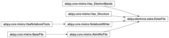
class abipy.electrons.eskw.EskwFile(filepath)

Bases: abipy.core.mixins.AbinitNcFile, abipy.core.mixins.Has_Structure, abipy.core.mixins.Has_ElectronBands, abipy.core.mixins.NotebookWriter

This file contains the (star-function) interpolated band structure produced by Abinit. It’s similar to the GSR file but it does not contain the header and energies.

Usage example:

with EskwFile("foo_ESKW.nc") as eskw:
    eskw.ebands.plot()

Inheritance Diagram

classmethod from_file(filepath)

Initialize the object from a netcdf file.

einterp()

band_block()

to_string(verbose=0)

String representation.

close()

Close the file.

property ebands

abipy.electrons.ebands.ElectronBands object.

property structure

abipy.core.structure.Structure object.

params()

OrderedDict with parameters that might be subject to convergence studies.

yield_figs(**kwargs)

This function generates a predefined list of matplotlib figures with minimal input from the user.

write_notebook(nbpath=None)

Write a jupyter notebook to nbpath. If nbpath is None, a temporay file in the current working directory is created. Return path to the notebook.

bse Module

Classes for the analysis of BSE calculations

class abipy.electrons.bse.DielectricFunction(structure, qpoints, wmesh, emacros_q, info)

Bases: object

This object stores the frequency-dependent macroscopic dielectric function computed for different q-directions in reciprocal space.

to_string(verbose=0, with_info=False)

String representation.

property num_qpoints

Number of q-points.

property qfrac_coords

numpy.ndarray with the fractional coordinates of the q-points.

plot(ax=None, **kwargs)

Plot the MDF.

Parameters

ax – matplotlib.axes.Axes or None if a new figure should be created.

kwargs	Meaning
only_mean	True if only the averaged spectrum is wanted (default True)

Returns: matplotlib.figure.Figure

Keyword arguments controlling the display of the figure:

kwargs	Meaning
title	Title of the plot (Default: None).
show	True to show the figure (default: True).
savefig	“abc.png” or “abc.eps” to save the figure to a file.
size_kwargs	Dictionary with options passed to fig.set_size_inches e.g. size_kwargs=dict(w=3, h=4)
tight_layout	True to call fig.tight_layout (default: False)
ax_grid	True (False) to add (remove) grid from all axes in fig. Default: None i.e. fig is left unchanged.
ax_annotate	Add labels to subplots e.g. (a), (b). Default: False
fig_close	Close figure. Default: False.

plot_ax(ax, qpoint=None, **kwargs)

Helper function to plot data on the axis ax.

Parameters

• ax – matplotlib.axes.Axes

• qpoint – index of the q-point or abipy.core.kpoints.Kpoint object or None to plot emacro_avg.

• kwargs –

  Keyword arguments passed to matplotlib. Accepts also:

  cplx_mode:

  string defining the data to print (case-insensitive). Possible choices are

  • ”re” for real part

  • ”im” for imaginary part only.

  • ”abs’ for the absolute value

  Options can be concated with “-“.

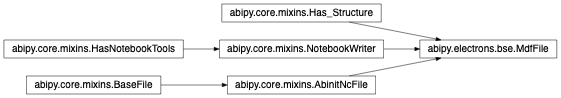
class abipy.electrons.bse.MdfFile(filepath)

Bases: abipy.core.mixins.AbinitNcFile, abipy.core.mixins.Has_Structure, abipy.core.mixins.NotebookWriter

Usage example:

with MdfFile("foo_MDF.nc") as mdf:
    mdf.plot_mdfs()

Inheritance Diagram

classmethod from_file(filepath)

Initialize the object from a Netcdf file

to_string(verbose=0)

String representation.

close()

Close the file.

structure()

abipy.core.structure.Structure object.

exc_mdf()

Excitonic macroscopic dieletric function.

rpanlf_mdf()

RPA dielectric function without local-field effects.

gwnlf_mdf()

RPA-GW dielectric function without local-field effects.

property qpoints

List of q-points.

property qfrac_coords

numpy.ndarray with the fractional coordinates of the q-points.

params()

Dictionary with the parameters that are usually tested for convergence. Used to build Pandas dataframes in Robots.

get_mdf(mdf_type='exc')

” Returns the macroscopic dielectric function.

plot_mdfs(cplx_mode='Im', mdf_type='all', qpoint=None, **kwargs)

Plot the macroscopic dielectric function.

Parameters

• cplx_mode –

  string defining the data to print (case-insensitive). Possible choices are

  • ”re” for real part

  • ”im” for imaginary part only.

  • ”abs’ for the absolute value

  Options can be concated with “-“.

• mdf_type –

  Select the type of macroscopic dielectric function. Possible choices are

  • ”exc” for the MDF with excitonic effects.

  • ”rpa” for RPA with KS energies.

  • ”gwrpa” for RPA with GW (or KS-corrected) results

  • ”all” if all types are wanted.

  Options can be concated with “-“.

• qpoint – index of the q-point or Kpoint object or None to plot emacro_avg.

get_tensor(mdf_type='exc')

Get the macroscopic dielectric tensor from the MDF.

yield_figs(**kwargs)

This function generates a predefined list of matplotlib figures with minimal input from the user. Used in abiview.py to get a quick look at the results.

write_notebook(nbpath=None)

Write a jupyter notebook to nbpath. If nbpath is None, a temporay file in the current working directory is created. Return path to the notebook.

class abipy.electrons.bse.MdfReader(path)

Bases: abipy.iotools.ETSF_Reader

This object reads data from the MDF.nc file produced by ABINIT.

Inheritance Diagram

property structure

abipy.core.structure.Structure object.

qpoints()

List of q-points (ndarray).

wmesh()

The frequency mesh in eV.

read_params()

Dictionary with the parameters of the run.

read_exc_mdf()

Returns the excitonic MDF.

read_rpanlf_mdf()

Returns the KS-RPA MDF without LF effects.

read_gwnlf_mdf()

Returns the GW-RPA MDF without LF effects.

class abipy.electrons.bse.MdfPlotter

Bases: object

Class for plotting Macroscopic dielectric functions.

Usage example:

plotter = MdfPlotter()
plotter.add_mdf("EXC", exc_mdf)
plotter.add_mdf("KS-RPA", rpanlf_mdf)
plotter.plot()

add_mdf(label, mdf)

Adds a DielectricFunction for plotting.

Parameters

• name – name for the MDF. Must be unique.

• mdf – DielectricFunction object.

plot(ax=None, cplx_mode='Im', qpoint=None, xlims=None, ylims=None, fontsize=12, **kwargs)

Get a matplotlib plot showing the MDFs.

Parameters

• ax – matplotlib.axes.Axes or None if a new figure should be created.

• cplx_mode – string defining the data to print (case-insensitive). Possible choices are re for the real part, im for imaginary part only. abs for the absolute value. Options can be concated with “-“.

• qpoint – index of the q-point or Kpoint object or None to plot emacro_avg.

• xlims – Set the data limits for the y-axis. Accept tuple e.g. (left, right) or scalar e.g. left. If left (right) is None, default values are used

• ylims – Same meaning as ylims but for the y-axis

• fontsize – Legend and label fontsize.

Return: matplotlib.figure.Figure

Keyword arguments controlling the display of the figure:

kwargs	Meaning
title	Title of the plot (Default: None).
show	True to show the figure (default: True).
savefig	“abc.png” or “abc.eps” to save the figure to a file.
size_kwargs	Dictionary with options passed to fig.set_size_inches e.g. size_kwargs=dict(w=3, h=4)
tight_layout	True to call fig.tight_layout (default: False)
ax_grid	True (False) to add (remove) grid from all axes in fig. Default: None i.e. fig is left unchanged.
ax_annotate	Add labels to subplots e.g. (a), (b). Default: False
fig_close	Close figure. Default: False.

class abipy.electrons.bse.MultipleMdfPlotter

Bases: object

Class for plotting multipe macroscopic dielectric functions extracted from several MDF.nc files

Usage example:

plotter = MultipleMdfPlotter()
plotter.add_mdf_file("file1", mdf_file1)
plotter.add_mdf_file("file2", mdf_file2)
plotter.plot()

MDF_TYPES = ('exc', 'rpa', 'gwrpa')

MDF_TYPECPLX2TEX = {'exc': {'abs': '$|\\varepsilon_{exc}|$', 'im': '$\\Im(\\varepsilon_{exc}$)', 're': '$\\Re(\\varepsilon_{exc})$'}, 'gwrpa': {'abs': '$|\\varepsilon_{gw-rpa}|$', 'im': '$\\Im(\\varepsilon_{gw-rpa})$', 're': '$\\Re(\\varepsilon_{gw-rpa})$'}, 'rpa': {'abs': '$|\\varepsilon_{rpa}|$', 'im': '$\\Im(\\varepsilon_{rpa})$', 're': '$\\Re(\\varepsilon_{rpa})$'}}

to_string(**kwargs)

String representation.

add_mdf_file(label, obj)

Extract dielectric functions from object obj, store data for plotting.

Parameters

• label – label associated to the MDF file. Must be unique.

• mdf – filepath or MdfFile object.

plot(mdf_type='exc', qview='avg', xlims=None, ylims=None, fontsize=8, **kwargs)

Plot all macroscopic dielectric functions (MDF) stored in the plotter

Parameters

• mdf_type – Selects the type of dielectric function. “exc” for the MDF with excitonic effects. “rpa” for RPA with KS energies. “gwrpa” for RPA with GW (or KS-corrected) results.

• qview – “avg” to plot the results averaged over q-points. “all” to plot q-point dependence.

• xlims – Set the data limits for the y-axis. Accept tuple e.g. (left, right) or scalar e.g. left. If left (right) is None, default values are used

• ylims – Same meaning as ylims but for the y-axis

• fontsize – fontsize for titles and legend.

Return: matplotlib.figure.Figure

Keyword arguments controlling the display of the figure:

kwargs	Meaning
title	Title of the plot (Default: None).
show	True to show the figure (default: True).
savefig	“abc.png” or “abc.eps” to save the figure to a file.
size_kwargs	Dictionary with options passed to fig.set_size_inches e.g. size_kwargs=dict(w=3, h=4)
tight_layout	True to call fig.tight_layout (default: False)
ax_grid	True (False) to add (remove) grid from all axes in fig. Default: None i.e. fig is left unchanged.
ax_annotate	Add labels to subplots e.g. (a), (b). Default: False
fig_close	Close figure. Default: False.

plot_mdftype_cplx(mdf_type, cplx_mode, qpoint=None, ax=None, xlims=None, ylims=None, with_legend=True, with_xlabel=True, with_ylabel=True, fontsize=8, **kwargs)

Helper function to plot data corresponds to mdf_type, cplx_mode, qpoint.

Parameters

• ax – matplotlib.axes.Axes or None if a new figure should be created.

• mdf_type –

• cplx_mode – string defining the data to print (case-insensitive). Possible choices are re for the real part, im for imaginary part only. abs for the absolute value.

• qpoint – index of the q-point or Kpoint object or None to plot emacro_avg.

• xlims – Set the data limits for the y-axis. Accept tuple e.g. (left, right) or scalar e.g. left. If left (right) is None, default values are used

• ylims – Same meaning as ylims but for the y-axis

• with_legend – True if legend should be added

• with_xlabel –

• with_ylabel –

• fontsize – Legend and label fontsize.

Return: matplotlib.figure.Figure

Keyword arguments controlling the display of the figure:

kwargs	Meaning
title	Title of the plot (Default: None).
show	True to show the figure (default: True).
savefig	“abc.png” or “abc.eps” to save the figure to a file.
size_kwargs	Dictionary with options passed to fig.set_size_inches e.g. size_kwargs=dict(w=3, h=4)
tight_layout	True to call fig.tight_layout (default: False)
ax_grid	True (False) to add (remove) grid from all axes in fig. Default: None i.e. fig is left unchanged.
ax_annotate	Add labels to subplots e.g. (a), (b). Default: False
fig_close	Close figure. Default: False.

ipw_select_plot()

Return an ipython widget with controllers to select the plot.

charges Module

HirshfeldCharges.

class abipy.electrons.charges.HirshfeldCharges(electron_charges, structure, reference_charges=None)

Bases: abipy.electrons.charges.Charges

Class representing the charges obtained from the Hirshfeld analysis. The charges refer to the total charges for each atom (i.e. Z-n_electrons). An eccess of electron has a negative charge

Inheritance Diagram

classmethod from_cut3d_outfile(filepath, structure)

Generates a HirshfeldCharges object from the outputfile of cut3d and a structure.

class abipy.electrons.charges.BaderCharges(electron_charges, structure, reference_charges=None)

Bases: abipy.electrons.charges.Charges

Class representing the charges obtained from the Bader analysis. TThe charges refer to the total charges for each atom (i.e. Z-n_electrons). An eccess of electron has a negative charge

Inheritance Diagram

classmethod from_files(density_path, pseudopotential_paths, with_core=True, workdir=None, **kwargs)

Uses the abinit density files and the bader executable from Henkelmann et al. to calculate the bader charges of the system. If pseudopotentials are given, the atomic charges will be extracted as well. See also [Henkelman2006].

The extraction of the core charges may be a time consuming calculation, depending on the size of the system. A tuning of the parameters may be required (see Density.ae_core_density_on_mesh).

Parameters

• density_path – Path to the abinit density file. Can be a fortran _DEN or a netCDF DEN.nc file. In case of fortran file, requires cut3d (version >= 8.6.1) for the convertion.

• pseudopotential_paths – Dictionary {element: pseudopotential path} for all the elements present in the system.

• with_core – Core charges will be extracted from the pseudopotentials with the Density.ae_core_density_on_mesh method. Requires pseudopotential_paths.

• workdir – Working directory. If None, a temporary directory is created.

• kwargs – arguments passed to the method Density.ae_core_density_on_mesh

Returns

An instance of BaderCharges

denpot Module

Density/potential files in netcdf/fortran format.

class abipy.electrons.denpot.DensityNcFile(filepath)

Bases: abipy.electrons.denpot._NcFileWithField

Netcdf File containing the electronic density.

Usage example:

with DensityNcFile("foo_DEN.nc") as ncfile:
    ncfile.density
    ncfile.ebands.plot()

Inheritance Diagram

field_name = 'density'

density()

Density object.

to_string(verbose=0)

String representation.

write_chgcar(filename=None)

Write density in CHGCAR format. Return ChgCar instance.

write_xsf(filename=None)

Write density in XSF format (xcrysden)

write_cube(filename=None, spin='total')

Write density in CUBE format.

class abipy.electrons.denpot.VhartreeNcFile(filepath)

Bases: abipy.electrons.denpot._NcFileWithField

Inheritance Diagram

field_name = 'vh'

vh()

Hartree potential.

class abipy.electrons.denpot.VxcNcFile(filepath)

Bases: abipy.electrons.denpot._NcFileWithField

Inheritance Diagram

field_name = 'vxc'

vxc()

XC potential.

class abipy.electrons.denpot.VhxcNcFile(filepath)

Bases: abipy.electrons.denpot._NcFileWithField

Inheritance Diagram

field_name = 'vhxc'

vhxc()

Hartree + XC potential.

class abipy.electrons.denpot.PotNcFile(filepath)

Bases: abipy.electrons.denpot._NcFileWithField

POT file produced by the GS part containing the total KS potential in real space.

Inheritance Diagram

field_name = 'vks'

vks()

Hartree + XC potential + sum of local pseudo-potential terms.

ebands Module

Classes to analyse electronic structures.

class abipy.electrons.ebands.ElectronBands(structure, kpoints, eigens, fermie, occfacts, nelect, nspinor, nspden, nband_sk=None, smearing=None, linewidths=None)

Bases: abipy.core.mixins.Has_Structure

Object storing the electron band structure.

fermie

Fermi level in eV. Note that, if the band structure has been computed with a NSCF run, fermie corresponds to the fermi level obtained in the SCF run that produced the density used for the band structure calculation.

Inheritance Diagram

Error

alias of abipy.electrons.ebands.ElectronBandsError

pad_fermie = 0.001

classmethod from_file(filepath)

Initialize an instance of abipy.electrons.ebands.ElectronBands from the netCDF file filepath.

classmethod from_binary_string(bstring)

Build object from a binary string with the netcdf data. Useful for implementing GUIs in which widgets returns binary data.

classmethod from_dict(d)

Reconstruct object from the dictionary in MSONable format produced by as_dict.

as_dict()

Return dictionary with JSON serialization.

classmethod as_ebands(obj)

Return an instance of abipy.electrons.ebands.ElectronBands from a generic object obj. Supports:

• instances of cls

• files (string) that can be open with abiopen and that provide an ebands attribute.

• objects providing an ebands attribute

classmethod from_mpid(material_id, api_key=None, endpoint=None, nelect=None, has_timerev=True, nspinor=1, nspden=None, line_mode=True)

Read bandstructure data corresponding to a materials project material_id. and return Abipy ElectronBands object. Return None if bands are not available.

Parameters

• material_id (str) – Materials Project material_id (a string, e.g., mp-1234).

• api_key (str) – A String API key for accessing the MaterialsProject REST interface. Please apply on the Materials Project website for one. If this is None, the code will check if there is a PMG_MAPI_KEY in your .pmgrc.yaml. If so, it will use that environment This makes easier for heavy users to simply add this environment variable to their setups and MPRester can then be called without any arguments.

• endpoint (str) – Url of endpoint to access the MaterialsProject REST interface. Defaults to the standard Materials Project REST address, but can be changed to other urls implementing a similar interface.

• nelect – Number of electrons in the unit cell.

• nspinor – Number of spinor components.

• line_mode (bool) – If True, fetch a BandStructureSymmLine object (default). If False, return the uniform band structure.

to_json()

Returns a JSON string representation of the MSONable object.

property structure

abipy.core.structure.Structure object.

get_plotter_with(self_key, other_key, other_ebands)

Build and abipy.electrons.ebands.ElectronBandsPlotter from self and other, use self_key and other_key as keywords

property spins

Spin range

property nband

property kidxs

Range with the index of the k-points.

property eigens

Eigenvalues in eV. numpy.ndarray with shape [nspin, nkpt, mband].

property linewidths

linewidths in eV. numpy.ndarray with shape [nspin, nkpt, mband].

property has_linewidths

True if bands with linewidths.

property occfacts

Occupation factors. numpy.ndarray with shape [nspin, nkpt, mband].

property reciprocal_lattice

pymatgen.core.lattice.Lattice with the reciprocal lattice vectors in Angstrom.

property shape

Shape of the array with the eigenvalues.

property has_metallic_scheme

True if we are using a metallic scheme for occupancies.

set_fermie_to_vbm()

Set the Fermi energy to the valence band maximum (VBM). Useful when the initial fermie energy comes from a GS-SCF calculation that may underestimate the Fermi energy because e.g. the IBZ sampling is shifted whereas the true VMB is at Gamma.

Return: New fermi energy in eV.

set_fermie_from_edos(edos, nelect=None)

Set the Fermi level using the integrated DOS computed in edos.

Args:

edos: abipy.electrons.ebands.ElectronDos object. nelect: Number of electrons. If None, the number of electrons in self. is used

Return: New fermi energy in eV.

set_fermie(new_fermie)

Set the new fermi energy. Return new value

with_points_along_path(frac_bounds=None, knames=None, dist_tol=1e-12)

Build new abipy.electrons.ebands.ElectronBands object containing the k-points along the input k-path specified by frac_bounds. Useful to extract energies along a path from calculation performed in the IBZ.

Parameters

• frac_bounds – [M, 3] array with the vertexes of the k-path in reduced coordinates. If None, the k-path is automatically selected from the structure.

• knames – List of strings with the k-point labels defining the k-path. It has precedence over frac_bounds.

• dist_tol – A point is considered to be on the path if its distance from the line is less than dist_tol.

Returns

namedtuple with the following attributes:

ebands: |ElectronBands| object.
ik_new2prev: Correspondence between the k-points in the new ebands and the kpoint
    of the previous band structure (self).

classmethod empty_with_ibz(ngkpt, structure, fermie, nelect, nsppol, nspinor, nspden, mband, shiftk=(0, 0, 0), kptopt=1, smearing=None, linewidths=None)

get_dict4pandas(with_geo=True, with_spglib=True)

Return a OrderedDict with the most important parameters:

• Chemical formula and number of atoms.

• Lattice lengths, angles and volume.

• The spacegroup number computed by Abinit (set to None if not available).

• The spacegroup number and symbol computed by spglib (set to None not with_spglib).

Useful to construct pandas DataFrames

Parameters

• with_geo – True if structure info should be added to the dataframe

• with_spglib – If True, spglib is invoked to get the spacegroup symbol and number.

has_bzmesh()

True if the k-point sampling is homogeneous.

has_bzpath()

True if the bands are computed on a k-path.

kptopt()

The value of the kptopt input variable.

has_timrev()

True if time-reversal symmetry is used in the BZ sampling.

supports_fermi_surface()

True if the kpoints used for the energies can be employed to visualize Fermi surface. Fermi surface viewers require gamma-centered k-mesh.

kindex(kpoint)

The index of the k-point in the internal list of k-points. Accepts: abipy.core.kpoints.Kpoint instance or integer.

skb_iter()

Iterator over (spin, k, band) indices.

deepcopy()

Deep copy of the ElectronBands object.

degeneracies(spin, kpoint, bands_range, tol_ediff=0.001)

Returns a list with the indices of the degenerate bands.

Parameters

• spin – Spin index.

• kpoint – K-point index or abipy.core.kpoints.Kpoint object

• bands_range – List of band indices to analyze.

• tol_ediff – Tolerance on the energy difference (in eV)

Returns

List of tuples [(e0, bands_e0), (e1, bands_e1, ….] Each tuple stores the degenerate energy and a list with the band indices. The band structure of silicon at Gamma, for example, will produce something like: [(-6.3, [0]), (5.6, [1, 2, 3]), (8.1, [4, 5, 6])]

enemin(spin=None, band=None)

Compute the minimum of the eigenvalues.

enemax(spin=None, band=None)

Compute the maximum of the eigenvalues.

dispersionless_states(erange=None, deltae=0.05, kfact=0.9)

This function detects dispersionless states. A state is dispersionless if there are more that (nkpt * kfact) energies in the energy intervale [e0 - deltae, e0 + deltae]

Parameters

• range to be analyzed in the form [emin (erange=Energy) –

• emax] –

• deltae – Defines the energy interval in eV around the KS eigenvalue.

• kfact – Can be used to change the criterion used to detect dispersionless states.

Returns

List of Electron objects. Each item contains information on the energy, the occupation and the location of the dispersionless band.

get_dataframe(e0='fermie')

Return a pandas.DataFrame with the following columns:

[‘spin’, ‘kidx’, ‘band’, ‘eig’, ‘occ’, ‘kpoint’]

where:

Column	Meaning
spin	spin index
kidx	k-point index
band	band index
eig	KS eigenvalue in eV.
occ	Occupation of the state.
kpoint	Kpoint object

Parameters

e0 – Option used to define the zero of energy in the band structure plot. Possible values: - fermie: shift all eigenvalues to have zero energy at the Fermi energy (self.fermie). - Number e.g e0=0.5: shift all eigenvalues to have zero energy at 0.5 eV - None: Don’t shift energies, equivalent to e0=0 The Fermi energy is saved in frame.fermie

boxplot(ax=None, e0='fermie', brange=None, swarm=False, **kwargs)

Use seaborn to draw a box plot to show distributions of eigenvalues with respect to the band index.

Parameters

• ax – matplotlib.axes.Axes or None if a new figure should be created.

• e0 – Option used to define the zero of energy in the band structure plot. Possible values: - fermie: shift all eigenvalues to have zero energy at the Fermi energy (self.fermie). - Number e.g e0 = 0.5: shift all eigenvalues to have zero energy at 0.5 eV. - None: Don’t shift energies, equivalent to e0 = 0.

• brange – Only bands such as brange[0] <= band_index < brange[1] are included in the plot.

• swarm – True to show the datapoints on top of the boxes

• kwargs – Keyword arguments passed to seaborn boxplot.

Return: matplotlib.figure.Figure

Keyword arguments controlling the display of the figure:

kwargs	Meaning
title	Title of the plot (Default: None).
show	True to show the figure (default: True).
savefig	“abc.png” or “abc.eps” to save the figure to a file.
size_kwargs	Dictionary with options passed to fig.set_size_inches e.g. size_kwargs=dict(w=3, h=4)
tight_layout	True to call fig.tight_layout (default: False)
ax_grid	True (False) to add (remove) grid from all axes in fig. Default: None i.e. fig is left unchanged.
ax_annotate	Add labels to subplots e.g. (a), (b). Default: False
fig_close	Close figure. Default: False.

classmethod from_pymatgen(pmg_bands, nelect, weights=None, has_timerev=True, ksampling=None, smearing=None, nspinor=1, nspden=None)

Convert a pymatgen bandstructure object to an Abipy abipy.electrons.ebands.ElectronBands object.

Parameters

• pmg_bands – pymatgen bandstructure object.

• nelect – Number of electrons in unit cell.

• weights – List of K-points weights (normalized to one, same order as pmg_bands.kpoints). This argument is optional but recommended when pmg_bands represents an IBZ sampling. If weights are not provided, Abipy methods requiring integrations in the BZ won’t work.

• has_timerev – True if time-reversal symmetry can be used.

• ksampling – dictionary with parameters passed to KSamplingInfo defining the k-points sampling. If None, hard-coded values are used. This argument is recommended if IBZ sampling.

• smearing – dictionary with parameters passed to Smearing If None, default hard-coded values are used.

• nspinor – Number of spinor components.

• nspden – Number of independent spin-density components. If None, nspden is automatically computed from nsppol

Warning

The Abipy bandstructure contains more information than the pymatgen object so the conversion is not complete, especially if you rely on the default values. Please read carefylly the docstring and the code and use the optional arguments to pass additional data required by AbiPy if you need a complete conversion.

to_pymatgen()

Return a pymatgen bandstructure object from an Abipy abipy.electrons.ebands.ElectronBands object.

property lomos

lomo states for each spin channel as a list of nsppol Electron.

lomo_sk(spin, kpoint)

Returns the LOMO state for the given spin, kpoint.

Parameters

• spin – Spin index

• kpoint – Index of the kpoint or abipy.core.kpoints.Kpoint object.

homo_sk(spin, kpoint)

Returns the HOMO state for the given spin, kpoint.

Parameters

• spin – Spin index

• kpoint – Index of the kpoint or abipy.core.kpoints.Kpoint object.

lumo_sk(spin, kpoint)

Returns the LUMO state for the given spin, kpoint.

Parameters

• spin – Spin index

• kpoint – Index of the kpoint or abipy.core.kpoints.Kpoint object.

property homos

homo states for each spin channel as a list of nsppol Electron.

property lumos

lumo states for each spin channel as a list of nsppol Electron.

property bandwidths

The bandwidth for each spin channel i.e. the energy difference (homo - lomo).

property fundamental_gaps

List of ElectronTransition with info on the fundamental gaps for each spin.

property direct_gaps

List of nsppol ElectronTransition with info on the direct gaps for each spin.

get_gaps_string(with_latex=True, unicode=False)

Return string with info about fundamental and direct gap (if not metallic scheme)

Parameters

• with_latex – True to get latex symbols for the gap names and formula else text.

• unicode – True to get unicode symbols for the formula else text.

get_kpoints_and_band_range_for_edges()

Find the reduced coordinates and the band indice associate to the band edges. Important: Call set_fermie_to_vbm() to set the Fermi level to the VBM before calling this method.

Return: (k0_list, effmass_bands_f90) (Fortran notation)

to_string(title=None, with_structure=True, with_kpoints=False, verbose=0)

Human-readable string with useful info such as band gaps, position of HOMO, LOMO…

Parameters

• with_structure – False if structural info shoud not be displayed.

• with_kpoints – False if k-point info shoud not be displayed.

• verbose – Verbosity level.

new_with_irred_kpoints(prune_step=None)

Return a new abipy.electrons.ebands.ElectronBands object in which only the irreducible k-points are kept. This method is mainly used to prepare the band structure interpolation as the interpolator will likely fail if the input k-path contains symmetrical k-points.

Parameters

• prune_step – Optional argument used to select a subset of the irreducible points found.

• prune_step is None (If) –

• irreducible k-points are used. (all) –

spacing(axis=None)

Compute the statistical parameters of the energy spacing, i.e. e[b+1] - e[b]

Returns

namedtuple with the statistical parameters in eV

statdiff(other, axis=None, numpy_op=<ufunc 'absolute'>)

Compare the eigenenergies of two bands and compute the statistical parameters: mean, standard deviation, min and max The bands are aligned wrt to their fermi level.

Parameters

• other – abipy.electrons.ebands.ElectronBands object.

• axis – Axis along which the statistical parameters are computed. The default is to compute the parameters of the flattened array.

• numpy_op – Numpy function to apply to the difference of the eigenvalues. The default computes |self.eigens - other.eigens|.

Returns

namedtuple with the statistical parameters in eV

ipw_edos_widget()

Return an ipython widget with controllers to compute the electron DOS.

get_edos(method='gaussian', step=0.1, width=0.2)

Compute the electronic DOS on a linear mesh.

Parameters

• method – String defining the method for the computation of the DOS.

• step – Energy step (eV) of the linear mesh.

• width – Standard deviation (eV) of the gaussian.

Returns: abipy.electrons.ebands.ElectronDos object.

compare_gauss_edos(widths, step=0.1)

Compute the electronic DOS with the Gaussian method for different values of the broadening. Return plotter object.

Parameters

• widths – List with the tandard deviation (eV) of the gaussian.

• step – Energy step (eV) of the linear mesh.

Return: abipy.electrons.ebands.ElectronDosPlotter

plot_transitions(omega_ev, qpt=(0, 0, 0), atol_ev=0.1, atol_kdiff=0.0001, ylims=None, ax=None, alpha=0.4, **kwargs)

Plot energy bands with arrows signaling possible k –> k + q indipendent-particle transitions of energy omega_ev connecting occupied to empty states.

Parameters

• omega_ev – Transition energy in eV.

• qpt – Q-point in reduced coordinates.

• atol_ev – Absolute tolerance for energy difference in eV

• atol_kdiff – Tolerance used to compare k-points.

• ylims – Set the data limits for the y-axis. Accept tuple e.g. (left, right) or scalar e.g. left. If left (right) is None, default values are used

• alpha – The alpha blending value, between 0 (transparent) and 1 (opaque)

• ax – matplotlib.axes.Axes or None if a new figure should be created.

Returns: matplotlib.figure.Figure

Keyword arguments controlling the display of the figure:

kwargs	Meaning
title	Title of the plot (Default: None).
show	True to show the figure (default: True).
savefig	“abc.png” or “abc.eps” to save the figure to a file.
size_kwargs	Dictionary with options passed to fig.set_size_inches e.g. size_kwargs=dict(w=3, h=4)
tight_layout	True to call fig.tight_layout (default: False)
ax_grid	True (False) to add (remove) grid from all axes in fig. Default: None i.e. fig is left unchanged.
ax_annotate	Add labels to subplots e.g. (a), (b). Default: False
fig_close	Close figure. Default: False.

get_ejdos(spin, valence, conduction, method='gaussian', step=0.1, width=0.2, mesh=None)

Compute the join density of states at q == 0.

\(\sum_{kbv} f_{vk} (1 - f_{ck}) \delta(\omega - E_{ck} + E_{vk})\)

Warning

The present implementation assumes an energy gap

Parameters

• spin – Spin index.

• valence – Int or iterable with the valence indices.

• conduction – Int or iterable with the conduction indices.

• method (str) – String defining the integraion method.

• step – Energy step (eV) of the linear mesh.

• width – Standard deviation (eV) of the gaussian.

• mesh – Frequency mesh to use. If None, the mesh is computed automatically from the eigenvalues.

Returns: abipy.core.func1d.Function1D object.

plot_ejdosvc(vrange, crange, method='gaussian', step=0.1, width=0.2, colormap='jet', cumulative=True, ax=None, alpha=0.7, fontsize=12, **kwargs)

Plot the decomposition of the joint-density of States (JDOS).

Warning

The present implementation assumes an energy gap

Parameters

• vrange – Int or Iterable with the indices of the valence bands to consider.

• crange – Int or Iterable with the indices of the conduction bands to consider.

• method – String defining the method.

• step – Energy step (eV) of the linear mesh.

• width – Standard deviation (eV) of the gaussian.

• colormap – Have a look at the colormaps here and decide which one you like: http://matplotlib.sourceforge.net/examples/pylab_examples/show_colormaps.html

• cumulative – True for cumulative plots (default).

• ax – matplotlib.axes.Axes or None if a new figure should be created.

• alpha – The alpha blending value, between 0 (transparent) and 1 (opaque)

• fontsize – fontsize for legends and titles

Returns: matplotlib.figure.Figure

Keyword arguments controlling the display of the figure:

kwargs	Meaning
title	Title of the plot (Default: None).
show	True to show the figure (default: True).
savefig	“abc.png” or “abc.eps” to save the figure to a file.
size_kwargs	Dictionary with options passed to fig.set_size_inches e.g. size_kwargs=dict(w=3, h=4)
tight_layout	True to call fig.tight_layout (default: False)
ax_grid	True (False) to add (remove) grid from all axes in fig. Default: None i.e. fig is left unchanged.
ax_annotate	Add labels to subplots e.g. (a), (b). Default: False
fig_close	Close figure. Default: False.

apply_scissors(scissors)

Modify the band structure with the scissors operator.

Parameters

scissors – An instance of Scissors.

Returns

New instance of abipy.electrons.ebands.ElectronBands with modified energies.

plot(spin=None, band_range=None, klabels=None, e0='fermie', ax=None, ylims=None, points=None, with_gaps=False, max_phfreq=None, fontsize=8, **kwargs)

Plot the electronic band structure with matplotlib.

Parameters

• spin – Spin index. None to plot both spins.

• band_range – Tuple specifying the minimum and maximum band to plot (default: all bands are plotted)

• klabels – dictionary whose keys are tuple with the reduced coordinates of the k-points. The values are the labels. e.g. klabels = {(0.0,0.0,0.0): "$\Gamma$", (0.5,0,0):"L"}.

• e0 – Option used to define the zero of energy in the band structure plot. Possible values: - fermie: shift all eigenvalues to have zero energy at the Fermi energy (self.fermie). - Number e.g e0=0.5: shift all eigenvalues to have zero energy at 0.5 eV - None: Don’t shift energies, equivalent to e0=0

• ax – matplotlib.axes.Axes or None if a new figure should be created.

• ylims – Set the data limits for the y-axis. Accept tuple e.g. (left, right) or scalar e.g. left. If left (right) is None, default values are used

• points – Marker object with the position and the size of the marker. Used for plotting purpose e.g. QP energies, energy derivatives…

• with_gaps –

  True to add markers and arrows showing the fundamental and the direct gap. IMPORTANT: If the gaps are now showed correctly in a non-magnetic semiconductor,

  call ebands.set_fermie_to_vbm() to align the Fermi level at the top of the valence bands before executing `ebands.plot(). The Fermi energy stored in the object, indeed, comes from the GS calculation that produced the DEN file. If the k-mesh used for the GS and the CBM is e.g. at Gamma, the Fermi energy will be underestimated and a manual aligment is needed.

• max_phfreq – Max phonon frequency in eV to activate scatterplot showing possible phonon absorption/emission processes based on energy-conservation alone. All final states whose energy is within +- max_phfreq of the initial state are included. By default, the four electronic states defining the fundamental and the direct gaps are considered as initial state (not available for metals).

• fontsize – fontsize for legends and titles

Returns: matplotlib.figure.Figure

Keyword arguments controlling the display of the figure:

kwargs	Meaning
title	Title of the plot (Default: None).
show	True to show the figure (default: True).
savefig	“abc.png” or “abc.eps” to save the figure to a file.
size_kwargs	Dictionary with options passed to fig.set_size_inches e.g. size_kwargs=dict(w=3, h=4)
tight_layout	True to call fig.tight_layout (default: False)
ax_grid	True (False) to add (remove) grid from all axes in fig. Default: None i.e. fig is left unchanged.
ax_annotate	Add labels to subplots e.g. (a), (b). Default: False
fig_close	Close figure. Default: False.

plotly(spin=None, band_range=None, klabels=None, e0='fermie', fig=None, rcd=None, ylims=None, points=None, with_gaps=False, max_phfreq=None, fontsize=12, **kwargs)

Plot the electronic band structure with plotly.

Parameters

• spin – Spin index. None to plot both spins.

• band_range – Tuple specifying the minimum and maximum band to plot (default: all bands are plotted)

• klabels – dictionary whose keys are tuple with the reduced coordinates of the k-points. The values are the labels. e.g. klabels = {(0.0,0.0,0.0): "$\Gamma$", (0.5,0,0):"L"}.

• e0 – Option used to define the zero of energy in the band structure plot. Possible values: - fermie: shift all eigenvalues to have zero energy at the Fermi energy (self.fermie). - Number e.g e0=0.5: shift all eigenvalues to have zero energy at 0.5 eV - None: Don’t shift energies, equivalent to e0=0

• fig – plotly figure or None if a new figure should be created.

• rcd – PlotlyRowColDesc object used when fig is not None to specify the (row, col) of the subplot in the grid.

• ylims – Set the data limits for the y-axis. Accept tuple e.g. (left, right)

• points – Marker object with the position and the size of the marker. Used for plotting purpose e.g. QP energies, energy derivatives.

• with_gaps – True to add markers and arrows showing the fundamental and the direct gap. IMPORTANT: If the gaps are now showed correctly in a non-magnetic semiconductor, call ebands.set_fermie_to_vbm() to align the Fermi level at the top of the valence bands before executing `ebands.plot(). The Fermi energy stored in the object, indeed, comes from the GS calculation that produced the DEN file. If the k-mesh used for the GS and the CBM is e.g. at Gamma, the Fermi energy will be underestimated and a manual aligment is needed.

• max_phfreq – Max phonon frequency in eV to activate scatterplot showing possible phonon absorption/emission processes based on energy-conservation alone. All final states whose energy is within +- max_phfreq of the initial state are included. By default, the four electronic states defining the fundamental and the direct gaps are considered as initial state (not available for metals).

• fontsize – fontsize for legends and titles

• kwargs – Passed to fig.add_scatter method.

Returns: plotly.graph_objects.Figure

Keyword arguments controlling the display of the figure: ================ ==================================================================== kwargs Meaning ================ ==================================================================== title Title of the plot (Default: None). show True to show the figure (default: True). hovormode True to show the hover info (default: False) savefig “abc.png” , “abc.jpeg” or “abc.webp” to save the figure to a file. write_json Write plotly figure to write_json JSON file.

Inside jupyter-lab, one can right-click the write_json file from the file menu and open with “Plotly Editor”. Make some changes to the figure, then use the file menu to save the customized plotly plot. Requires jupyter labextension install jupyterlab-chart-editor. See https://github.com/plotly/jupyterlab-chart-editor

renderer (str or None (default None)) –

A string containing the names of one or more registered renderers (separated by ‘+’ characters) or None. If None, then the default renderers specified in plotly.io.renderers.default are used. See https://plotly.com/python-api-reference/generated/plotly.graph_objects.Figure.html

config (dict) A dict of parameters to configure the figure. The defaults are set in plotly.js. chart_studio True to push figure to chart_studio server. Requires authenticatios.

Default: False.

plot_scatter3d(band, spin=0, e0='fermie', colormap='jet', ax=None, **kwargs)

Use matplotlib scatter3D to produce a scatter plot of the eigenvalues in 3D. The color of the points gives the energy of the state wrt to the Fermi level.

Parameters

• band – Band index

• spin – Spin index.

• e0 – Option used to define the zero of energy in the band structure plot. Possible values: - fermie: shift all eigenvalues to have zero energy at the Fermi energy (self.fermie). - Number e.g e0 = 0.5: shift all eigenvalues to have zero energy at 0.5 eV - None: Don’t shift energies, equivalent to e0 = 0.

• colormap – Have a look at the colormaps here and decide which one you like: <http://matplotlib.sourceforge.net/examples/pylab_examples/show_colormaps.html>

• ax – matplotlib Axes3D or None if a new figure should be created.

Keyword arguments controlling the display of the figure:

kwargs	Meaning
title	Title of the plot (Default: None).
show	True to show the figure (default: True).
savefig	“abc.png” or “abc.eps” to save the figure to a file.
size_kwargs	Dictionary with options passed to fig.set_size_inches e.g. size_kwargs=dict(w=3, h=4)
tight_layout	True to call fig.tight_layout (default: False)
ax_grid	True (False) to add (remove) grid from all axes in fig. Default: None i.e. fig is left unchanged.
ax_annotate	Add labels to subplots e.g. (a), (b). Default: False
fig_close	Close figure. Default: False.

decorate_ax(ax, **kwargs)

Add k-labels, title and unit name to axis ax.

Parameters

• title –

• fontsize –

• klabels –

• klabel_size –

decorate_plotly(fig, **kwargs)

Add q-labels and unit name to figure fig. Use units=”” to add k-labels without unit name. :param klabels: :param klabel_size: :param iax: An int, use iax=n to decorate the nth axis when the fig has subplots.

get_e0(e0)

e0: Option used to define the zero of energy in the band structure plot. Possible values:

• fermie: shift all eigenvalues to have zero energy at the Fermi energy (self.fermie).

• Number e.g e0 = 0.5: shift all eigenvalues to have zero energy at 0.5 eV

• None: Don’t shift energies, equivalent to e0 = 0.

plot_ax(ax, e0, spin=None, band=None, **kwargs)

Helper function to plot the energies for (spin, band) on the axis ax with matplotlib..

Parameters

• ax – matplotlib.axes.Axes.

• e0 – Option used to define the zero of energy in the band structure plot.

• spin – Spin index. If None, all spins are plotted.

• band – Band index, If None, all bands are plotted.

• kwargs – Passed to ax.plot

Return: matplotlib lines

plotly_traces(fig, e0, rcd=None, spin=None, band=None, showlegend=False, line_opts=None, **kwargs)

Helper function to plot the energies for (spin, band) on figure fig.

Parameters

• fig – plotly.graph_objects.Figure.

• e0 – Option used to define the zero of energy in the band structure plot.

• rcd – PlotlyRowColDesc object used when fig is not None to specify the (row, col) of the subplot in the grid.

• spin – Spin index. If None, all spins are plotted.

• band – Band index, If None, all bands are plotted.

• showlegend – Determines whether or not an item corresponding to this trace is shown in the legend.

• kwargs – Passed to fig.add_scatter method.

plot_with_edos(edos, klabels=None, ax_list=None, e0='fermie', points=None, with_gaps=False, max_phfreq=None, ylims=None, width_ratios=(2, 1), **kwargs)

Plot the band structure and the DOS with matplotlib.

Parameters

• edos – An instance of abipy.electrons.ebands.ElectronDos.

• klabels – dictionary whose keys are tuple with the reduced coordinates of the k-points. The values are the labels. e.g. klabels = {(0.0,0.0,0.0): "$\Gamma$", (0.5,0,0): "L"}.

• ax_list – The axes for the bandstructure plot and the DOS plot. If ax_list is None, a new figure is created and the two axes are automatically generated.

• ylims – Set the data limits for the y-axis. Accept tuple e.g. (left, right) or scalar e.g. left. If left (right) is None, default values are used

• e0 –

  Option used to define the zero of energy in the band structure plot. Possible values:

  * ``fermie``: shift all eigenvalues and the DOS to have zero energy at the Fermi energy.
     Note that, by default, the Fermi energy is taken from the band structure object
     i.e. the Fermi energy computed at the end of the SCF file that produced the density.
     This should be ok in semiconductors. In metals, however, a better value of the Fermi energy
     can be obtained from the DOS provided that the k-sampling for the DOS is much denser than
     the one used to compute the density. See ``edos_fermie``.
  * ``edos_fermie``: Use the Fermi energy computed from the DOS to define the zero of energy in both subplots.
  *  Number e.g ``e0 = 0.5``: shift all eigenvalues to have zero energy at 0.5 eV
  *  None: Don't shift energies, equivalent to ``e0 = 0``
  

• points – Marker object with the position and the size of the marker. Used for plotting purpose e.g. QP energies, energy derivatives…

• with_gaps – True to add markers and arrows showing the fundamental and the direct gap.

• max_phfreq – Max phonon frequency in eV to activate scatterplot showing possible phonon absorption/emission processes based on energy-conservation alone. All final states whose energy is within +- max_phfreq of the initial state are included. By default, the four electronic states defining the fundamental and the direct gaps are considered as initial state (not available for metals).

• width_ratios – Defines the ratio between the band structure plot and the dos plot.

Return: matplotlib.figure.Figure

Keyword arguments controlling the display of the figure:

kwargs	Meaning
title	Title of the plot (Default: None).
show	True to show the figure (default: True).
savefig	“abc.png” or “abc.eps” to save the figure to a file.
size_kwargs	Dictionary with options passed to fig.set_size_inches e.g. size_kwargs=dict(w=3, h=4)
tight_layout	True to call fig.tight_layout (default: False)
ax_grid	True (False) to add (remove) grid from all axes in fig. Default: None i.e. fig is left unchanged.
ax_annotate	Add labels to subplots e.g. (a), (b). Default: False
fig_close	Close figure. Default: False.

plotly_with_edos(edos, klabels=None, fig=None, e0='fermie', points=None, with_gaps=False, max_phfreq=None, ylims=None, width_ratios=(2, 1), **kwargs)

Plot the band structure and the DOS with plotly.

Parameters

• edos – An instance of abipy.electrons.ebands.ElectronDos.

• klabels – dictionary whose keys are tuple with the reduced coordinates of the k-points. The values are the labels. e.g. klabels = {(0.0,0.0,0.0): "$\Gamma$", (0.5,0,0): "L"}.

• fig – The plotly.graph_objects.Figure with two distinct plots for the bandstructure plot and the DOS plot. If fig is None, a new figure is created.

• ylims – Set the data limits for the y-axis. Accept tuple e.g. (left, right)

• e0 –

  Option used to define the zero of energy in the band structure plot. Possible values:

  * ``fermie``: shift all eigenvalues and the DOS to have zero energy at the Fermi energy.
     Note that, by default, the Fermi energy is taken from the band structure object
     i.e. the Fermi energy computed at the end of the SCF file that produced the density.
     This should be ok in semiconductors. In metals, however, a better value of the Fermi energy
     can be obtained from the DOS provided that the k-sampling for the DOS is much denser than
     the one used to compute the density. See ``edos_fermie``.
  * ``edos_fermie``: Use the Fermi energy computed from the DOS to define the zero of energy in both subplots.
  *  Number e.g ``e0 = 0.5``: shift all eigenvalues to have zero energy at 0.5 eV
  *  None: Don't shift energies, equivalent to ``e0 = 0``
  

• points – Marker object with the position and the size of the marker. Used for plotting purpose e.g. QP energies, energy derivatives…

• with_gaps – True to add markers and arrows showing the fundamental and the direct gap.

• max_phfreq – Max phonon frequency in eV to activate scatterplot showing possible phonon absorption/emission processes based on energy-conservation alone. All final states whose energy is within +- max_phfreq of the initial state are included. By default, the four electronic states defining the fundamental and the direct gaps are considered as initial state (not available for metals).

• width_ratios – Defines the ratio between the band structure plot and the dos plot.

Return: plotly.graph_objects.Figure

Keyword arguments controlling the display of the figure: ================ ==================================================================== kwargs Meaning ================ ==================================================================== title Title of the plot (Default: None). show True to show the figure (default: True). hovormode True to show the hover info (default: False) savefig “abc.png” , “abc.jpeg” or “abc.webp” to save the figure to a file. write_json Write plotly figure to write_json JSON file.

Inside jupyter-lab, one can right-click the write_json file from the file menu and open with “Plotly Editor”. Make some changes to the figure, then use the file menu to save the customized plotly plot. Requires jupyter labextension install jupyterlab-chart-editor. See https://github.com/plotly/jupyterlab-chart-editor

renderer (str or None (default None)) –

A string containing the names of one or more registered renderers (separated by ‘+’ characters) or None. If None, then the default renderers specified in plotly.io.renderers.default are used. See https://plotly.com/python-api-reference/generated/plotly.graph_objects.Figure.html

config (dict) A dict of parameters to configure the figure. The defaults are set in plotly.js. chart_studio True to push figure to chart_studio server. Requires authenticatios.

Default: False.

plot_lws_vs_e0(ax=None, e0='fermie', function=<function ElectronBands.<lambda>>, exchange_xy=False, xlims=None, ylims=None, fontsize=12, **kwargs)

Plot electronic linewidths vs KS energy with matplotlib.

Parameters

• ax – matplotlib.axes.Axes or None if a new figure should be created.

• e0 – Option used to define the zero of energy in the band structure plot. Possible values: - fermie: shift all eigenvalues to have zero energy at the Fermi energy (self.fermie). - Number e.g e0=0.5: shift all eigenvalues to have zero energy at 0.5 eV - None: Don’t shift energies, equivalent to e0=0

• function – Apply this function to the values before plotting

• exchange_xy – True to exchange x-y axis.

• xlims – Set the data limits for the x-axis or the y-axis. Accept tuple e.g. (left, right) or scalar e.g. left. If left (right) is None, default values are used

• ylims – Set the data limits for the x-axis or the y-axis. Accept tuple e.g. (left, right) or scalar e.g. left. If left (right) is None, default values are used

• fontsize – fontsize for titles and legend.

Returns: matplotlib.figure.Figure

Keyword arguments controlling the display of the figure:

kwargs	Meaning
title	Title of the plot (Default: None).
show	True to show the figure (default: True).
savefig	“abc.png” or “abc.eps” to save the figure to a file.
size_kwargs	Dictionary with options passed to fig.set_size_inches e.g. size_kwargs=dict(w=3, h=4)
tight_layout	True to call fig.tight_layout (default: False)
ax_grid	True (False) to add (remove) grid from all axes in fig. Default: None i.e. fig is left unchanged.
ax_annotate	Add labels to subplots e.g. (a), (b). Default: False
fig_close	Close figure. Default: False.

to_xmgrace(filepath)

Write xmgrace file with band structure energies and labels for high-symmetry k-points.

Parameters

filepath – String with filename or stream.

to_bxsf(filepath)

Export the full band structure to filepath in BXSF format suitable for the visualization of isosurfaces with xcrysden (xcrysden –bxsf FILE). Require k-points in IBZ and gamma-centered k-mesh.

get_ebands3d()

derivatives(spin, band, order=1, acc=4)

Compute the derivative of the eigenvalues wrt to k.

Parameters

• spin – Spin index

• band – Band index

• order –

• acc –

Returns:

effective_masses(spin, band, acc=4)

Compute the effective masses for the given spin and band index. Use finite difference with accuracy acc.

Returns

numpy.ndarray of size self.nkpt with effective masses.

get_effmass_line(spin, kpoint, band, acc=4)

Compute the effective masses along a k-line. Requires band energies on a k-path.

Parameters

• spin – Spin index.

• kpoint – integer, list of fractional coordinates or abipy.core.kpoints.Kpoint object.

• band – Band index.

• acc – accuracy

interpolate(lpratio=5, knames=None, vertices_names=None, line_density=20, kmesh=None, is_shift=None, bstart=0, bstop=None, filter_params=None, verbose=0)

Interpolate energies in k-space along a k-path and, optionally, in the IBZ for DOS calculations. Note that the interpolation will likely fail if there are symmetrical k-points in the input set of k-points so it’s recommended to call this method with energies obtained in the IBZ.

Parameters

• lpratio – Ratio between the number of star functions and the number of ab-initio k-points. The default should be OK in many systems, larger values may be required for accurate derivatives.

• knames – List of strings with the k-point labels for the k-path. Has precedence over vertices_names.

• vertices_names – Used to specify the k-path for the interpolated band structure It’s a list of tuple, each tuple is of the form (kfrac_coords, kname) where kfrac_coords are the reduced coordinates of the k-point and kname is a string with the name of the k-point. Each point represents a vertex of the k-path. line_density defines the density of the sampling. If None, the k-path is automatically generated according to the point group of the system.

• line_density – Number of points in the smallest segment of the k-path. If 0, use list of k-points given in vertices_names

• kmesh – Used to activate the interpolation on the homogeneous mesh for DOS (uses spglib API). kmesh is given by three integers and specifies mesh numbers along reciprocal primitive axis.

• is_shift – three integers (spglib API). When is_shift is not None, the kmesh is shifted along the axis in half of adjacent mesh points irrespective of the mesh numbers. None means unshited mesh.

• bstart – Select the range of band to be used in the interpolation

• bstop – Select the range of band to be used in the interpolation

• filter_params – TO BE described.

• verbose – Verbosity level

Returns

namedtuple with the following attributes:

ebands_kpath: |ElectronBands| with the interpolated band structure on the k-path.
ebands_kmesh: |ElectronBands| with the interpolated band structure on the k-mesh.
    None if ``kmesh`` is not given.
interpolator: |SkwInterpolator| object.

get_collinear_mag()

Calculates the total collinear magnetization in Bohr magneton as the difference between the spin up and spin down densities.

Returns

the total magnetization.

Return type

float

class abipy.electrons.ebands.ElectronDos(mesh, spin_dos, nelect, fermie=None, spin_idos=None)

Bases: object

This object stores the electronic density of states. It is usually created by calling the get_edos method of abipy.electrons.ebands.ElectronBands.

to_string(verbose=0)

String representation.

classmethod as_edos(obj, edos_kwargs)

Return an instance of abipy.electrons.ebands.ElectronDos from a generic object obj. Supports:

• instances of cls

• files (string) that can be open with abiopen and that provide an ebands attribute.

• objects providing an ebands or get_edos attribute

Parameters

• edos_kwargs – optional dictionary with the options passed to get_edos to compute the electron DOS.

• when obj is not already an instance of cls. (Used) –

dos_idos(spin=None)

Returns DOS and IDOS for given spin. Total DOS and IDOS if spin is None.

find_mu(nelect, spin=None)

Finds the chemical potential given the number of electrons.

up_minus_down()

Function1D with dos_up - dos_down

get_e0(e0)

e0: Option used to define the zero of energy in the band structure plot. Possible values:

• fermie: shift all eigenvalues to have zero energy at the Fermi energy (self.fermie).

• Number e.g e0=0.5: shift all eigenvalues to have zero energy at 0.5 eV

• None: Don’t shift energies, equivalent to e0=0

plot_ax(ax, e0, spin=None, what='dos', fact=1.0, exchange_xy=False, **kwargs)

Helper function to plot the DOS data on the matplotlib axis ax.

Parameters

• ax – matplotlib.axes.Axes.

• e0 – Option used to define the zero of energy in the band structure plot.

• spin – selects the spin component, None for total DOS, IDOS.

• what – string selecting what will be plotted. “dos” for DOS, “idos” for IDOS

• fact – Multiplication factor for DOS/IDOS. Usually +-1 for spin DOS

• exchange_xy – True to exchange x-y axis.

• kwargs – Options passed to matplotlib ax.plot

Return: list of lines added to the axis ax.

plotly_traces(fig, e0, spin=None, what='dos', fact=1.0, exchange_xy=False, rcd=None, trace_name='', showlegend=False, line_opts=None, **kwargs)

Helper function to plot the DOS data on the fig with plotly.

Parameters

• fig – plotly.graph_objects.Figure.

• e0 – Option used to define the zero of energy in the band structure plot.

• spin – selects the spin component, None for total DOS, IDOS.

• what – string selecting what will be plotted. “dos” for DOS, “idos” for IDOS

• fact – Multiplication factor for DOS/IDOS. Usually +-1 for spin DOS

• exchange_xy – True to exchange x-y axis.

• rcd – PlotlyRowColDesc object used to specify the (row, col) of the subplot in the grid.

• trace_name – Name of the trace.

• showlegend – Determines whether or not an item corresponding to this trace is shown in the legend.

• line_opts – Dict of options passed to |plotly.graph_objects.scatter.Line|

• kwargs – Options passed to fig.add_scatter method.

plot(e0='fermie', spin=None, ax=None, exchange_xy=False, xlims=None, ylims=None, **kwargs)

Plot electronic DOS with matplotlib.

Parameters

• e0 – Option used to define the zero of energy in the band structure plot. Possible values: - fermie: shift all eigenvalues to have zero energy at the Fermi energy (self.fermie). - Number e.g e0 = 0.5: shift all eigenvalues to have zero energy at 0.5 eV - None: Don’t shift energies, equivalent to e0 = 0.

• spin – Selects the spin component, None if total DOS is wanted.

• ax – matplotlib.axes.Axes or None if a new figure should be created.

• exchange_xy – True to exchange x-y axis.

• xlims – Set the data limits for the x-axis. Accept tuple e.g. (left, right) or scalar e.g. left. If left (right) is None, default values are used

• ylims – Set data limits for the y-axis.

• kwargs – options passed to ax.plot.

Return: matplotlib.figure.Figure

Keyword arguments controlling the display of the figure:

kwargs	Meaning
title	Title of the plot (Default: None).
show	True to show the figure (default: True).
savefig	“abc.png” or “abc.eps” to save the figure to a file.
size_kwargs	Dictionary with options passed to fig.set_size_inches e.g. size_kwargs=dict(w=3, h=4)
tight_layout	True to call fig.tight_layout (default: False)
ax_grid	True (False) to add (remove) grid from all axes in fig. Default: None i.e. fig is left unchanged.
ax_annotate	Add labels to subplots e.g. (a), (b). Default: False
fig_close	Close figure. Default: False.

plotly(e0='fermie', spin=None, fig=None, exchange_xy=False, xlims=None, ylims=None, trace_name='', showlegend=False, **kwargs)

Plot electronic DOS with plotly.

Parameters

• e0 – Option used to define the zero of energy in the band structure plot. Possible values: - fermie: shift all eigenvalues to have zero energy at the Fermi energy (self.fermie). - Number e.g e0 = 0.5: shift all eigenvalues to have zero energy at 0.5 eV - None: Don’t shift energies, equivalent to e0 = 0.

• spin – Selects the spin component, None if total DOS is wanted.

• fig – plotly.graph_objects.Figure.

• exchange_xy – True to exchange x-y axis.

• xlims – Set the data limits for the x-axis. Accept tuple e.g. (left, right).

• ylims – Set the data limits for the y-axis. Accept tuple e.g. (left, right).

• trace_name – Name of the trace.

• showlegend – Determines whether or not an item corresponding to this trace is shown in the legend.

• kwargs – Options passed to fig.add_scatter method.

Return: plotly.graph_objects.Figure

Keyword arguments controlling the display of the figure: ================ ==================================================================== kwargs Meaning ================ ==================================================================== title Title of the plot (Default: None). show True to show the figure (default: True). hovormode True to show the hover info (default: False) savefig “abc.png” , “abc.jpeg” or “abc.webp” to save the figure to a file. write_json Write plotly figure to write_json JSON file.

Inside jupyter-lab, one can right-click the write_json file from the file menu and open with “Plotly Editor”. Make some changes to the figure, then use the file menu to save the customized plotly plot. Requires jupyter labextension install jupyterlab-chart-editor. See https://github.com/plotly/jupyterlab-chart-editor

renderer (str or None (default None)) –

A string containing the names of one or more registered renderers (separated by ‘+’ characters) or None. If None, then the default renderers specified in plotly.io.renderers.default are used. See https://plotly.com/python-api-reference/generated/plotly.graph_objects.Figure.html

config (dict) A dict of parameters to configure the figure. The defaults are set in plotly.js. chart_studio True to push figure to chart_studio server. Requires authenticatios.

Default: False.

plot_dos_idos(e0='fermie', ax_list=None, xlims=None, height_ratios=(1, 2), **kwargs)

Plot electronic DOS and Integrated DOS on two different subplots with matplotlib.

Parameters

• e0 – Option used to define the zero of energy in the band structure plot. Possible values: - fermie: shift all eigenvalues to have zero energy at the Fermi energy (self.fermie). - Number e.g e0 = 0.5: shift all eigenvalues to have zero energy at 0.5 eV - None: Don’t shift energies, equivalent to e0 = 0.

• ax_list – The axes for the DOS and IDOS plot. If ax_list is None, a new figure is created and the two axes are automatically generated.

• xlims – Set the data limits for the x-axis. Accept tuple e.g. (left, right) or scalar e.g. left. If left (right) is None, default values are used

• height_ratios –

• kwargs – options passed to plot_ax

Return: matplotlib.figure.Figure

Keyword arguments controlling the display of the figure:

kwargs	Meaning
title	Title of the plot (Default: None).
show	True to show the figure (default: True).
savefig	“abc.png” or “abc.eps” to save the figure to a file.
size_kwargs	Dictionary with options passed to fig.set_size_inches e.g. size_kwargs=dict(w=3, h=4)
tight_layout	True to call fig.tight_layout (default: False)
ax_grid	True (False) to add (remove) grid from all axes in fig. Default: None i.e. fig is left unchanged.
ax_annotate	Add labels to subplots e.g. (a), (b). Default: False
fig_close	Close figure. Default: False.

plotly_dos_idos(e0='fermie', fig=None, xlims=None, height_ratios=(1, 2), **kwargs)

Plot electronic DOS and Integrated DOS on two different subplots with plotly.

Parameters

• e0 – Option used to define the zero of energy in the band structure plot. Possible values: - fermie: shift all eigenvalues to have zero energy at the Fermi energy (self.fermie). - Number e.g e0 = 0.5: shift all eigenvalues to have zero energy at 0.5 eV - None: Don’t shift energies, equivalent to e0 = 0.

• fig – The plotly.graph_objects.Figure with two distinct plots for the DOS and IDOS plot. If fig is None, a new figure is created.

• xlims – Set the data limits for the x-axis. Accept tuple e.g. (left, right).

• height_ratios –

• kwargs – Options passed to plotly_traces method.

Return: plotly.graph_objects.Figure

Keyword arguments controlling the display of the figure: ================ ==================================================================== kwargs Meaning ================ ==================================================================== title Title of the plot (Default: None). show True to show the figure (default: True). hovormode True to show the hover info (default: False) savefig “abc.png” , “abc.jpeg” or “abc.webp” to save the figure to a file. write_json Write plotly figure to write_json JSON file.

Inside jupyter-lab, one can right-click the write_json file from the file menu and open with “Plotly Editor”. Make some changes to the figure, then use the file menu to save the customized plotly plot. Requires jupyter labextension install jupyterlab-chart-editor. See https://github.com/plotly/jupyterlab-chart-editor

renderer (str or None (default None)) –

A string containing the names of one or more registered renderers (separated by ‘+’ characters) or None. If None, then the default renderers specified in plotly.io.renderers.default are used. See https://plotly.com/python-api-reference/generated/plotly.graph_objects.Figure.html

config (dict) A dict of parameters to configure the figure. The defaults are set in plotly.js. chart_studio True to push figure to chart_studio server. Requires authenticatios.

Default: False.

plot_up_minus_down(e0='fermie', ax=None, xlims=None, **kwargs)

Plot Dos_up - Dow_down with matplotlib.

Parameters

• e0 – Option used to define the zero of energy in the band structure plot. Possible values: - fermie: shift all eigenvalues to have zero energy at the Fermi energy (self.fermie). - Number e.g e0 = 0.5: shift all eigenvalues to have zero energy at 0.5 eV - None: Don’t shift energies, equivalent to e0 = 0

• ax – matplotlib.axes.Axes or None if a new figure should be created.

• xlims – Set the data limits for the x-axis. Accept tuple e.g. (left, right) or scalar e.g. left. If left (right) is None, default values are used

• kwargs – options passed to ax.plot.

Return: matplotlib.figure.Figure

Keyword arguments controlling the display of the figure:

kwargs	Meaning
title	Title of the plot (Default: None).
show	True to show the figure (default: True).
savefig	“abc.png” or “abc.eps” to save the figure to a file.
size_kwargs	Dictionary with options passed to fig.set_size_inches e.g. size_kwargs=dict(w=3, h=4)
tight_layout	True to call fig.tight_layout (default: False)
ax_grid	True (False) to add (remove) grid from all axes in fig. Default: None i.e. fig is left unchanged.
ax_annotate	Add labels to subplots e.g. (a), (b). Default: False
fig_close	Close figure. Default: False.

plotly_up_minus_down(e0='fermie', fig=None, xlims=None, **kwargs)

Plot Dos_up - Dow_down with plotly.

Parameters

• e0 – Option used to define the zero of energy in the band structure plot. Possible values: - fermie: shift all eigenvalues to have zero energy at the Fermi energy (self.fermie). - Number e.g e0 = 0.5: shift all eigenvalues to have zero energy at 0.5 eV - None: Don’t shift energies, equivalent to e0 = 0

• fig – plotly.graph_objects.Figure or None if a new figure should be created.

• xlims – Set the data limits for the x-axis. Accept tuple e.g. (left, right).

• kwargs – Options passed to fig.add_scatter method.

Return: plotly.graph_objects.Figure

Keyword arguments controlling the display of the figure: ================ ==================================================================== kwargs Meaning ================ ==================================================================== title Title of the plot (Default: None). show True to show the figure (default: True). hovormode True to show the hover info (default: False) savefig “abc.png” , “abc.jpeg” or “abc.webp” to save the figure to a file. write_json Write plotly figure to write_json JSON file.

Inside jupyter-lab, one can right-click the write_json file from the file menu and open with “Plotly Editor”. Make some changes to the figure, then use the file menu to save the customized plotly plot. Requires jupyter labextension install jupyterlab-chart-editor. See https://github.com/plotly/jupyterlab-chart-editor

renderer (str or None (default None)) –

A string containing the names of one or more registered renderers (separated by ‘+’ characters) or None. If None, then the default renderers specified in plotly.io.renderers.default are used. See https://plotly.com/python-api-reference/generated/plotly.graph_objects.Figure.html

config (dict) A dict of parameters to configure the figure. The defaults are set in plotly.js. chart_studio True to push figure to chart_studio server. Requires authenticatios.

Default: False.

abipy.electrons.ebands.dataframe_from_ebands(ebands_objects, index=None, with_spglib=True)

Build a pandas dataframe with the most important results available in a list of band structures.

Parameters

• ebands_objects – List of objects that can be converted to structure. Support netcdf filenames or abipy.electrons.ebands.ElectronBands objects See ElectronBands.as_ebands for the complete list.

• index – Index of the dataframe.

• with_spglib – If True, spglib is invoked to get the spacegroup symbol and number.

Return: pandas.DataFrame

class abipy.electrons.ebands.ElectronBandsPlotter(key_ebands=None, key_edos=None, edos_kwargs=None)

Bases: abipy.core.mixins.NotebookWriter

Class for plotting electronic band structure and DOSes. Supports plots on the same graph or separated plots.

Usage example:

plotter = ElectronBandsPlotter()
plotter.add_ebands("foo-label", "foo_GSR.nc")
plotter.add_ebands("bar-label", "bar_WFK.nc")
fig = plotter.gridplot()

Dictionary with the mapping label –> edos.

Inheritance Diagram

add_plotter(other)

Merge two plotters, return new plotter.

to_string(func=<class 'str'>, verbose=0)

String representation.

get_ebands_frame(with_spglib=True)

Build a pandas.DataFrame with the most important results available in the band structures. Useful to analyze band-gaps.

property ebands_list

“List of abipy.electrons.ebands.ElectronBands objects.

property edoses_list

“List of abipy.electrons.ebands.ElectronDos objects.

iter_lineopt()

Generates matplotlib linestyles.

add_ebands(label, bands, edos=None, edos_kwargs=None)

Adds a band structure and optionally an edos to the plotter.

Parameters

• label – label for the bands. Must be unique.

• bands – abipy.electrons.ebands.ElectronBands object.

• edos – abipy.electrons.ebands.ElectronDos object.

• edos_kwargs – optional dictionary with the options passed to get_edos to compute the electron DOS. Used only if edos is not None and it’s not an abipy.electrons.ebands.ElectronDos instance.

bands_statdiff(ref=0)

Compare the reference bands with index ref with the other bands stored in the plotter.

yield_figs(**kwargs)

This function generates a predefined list of matplotlib figures with minimal input from the user.

combiplot(e0='fermie', ylims=None, width_ratios=(2, 1), fontsize=8, linestyle_dict=None, **kwargs)

Plot the band structure and the DOS on the same figure. Use gridplot to plot band structures on different figures.

Parameters

• e0 –

  Option used to define the zero of energy in the band structure plot. Possible values::

  • fermie: shift all eigenvalues to have zero energy at the Fermi energy (ebands.fermie)

    Note that, by default, the Fermi energy is taken from the band structure object i.e. the Fermi energy computed at the end of the SCF file that produced the density. This should be ok in semiconductors. In metals, however, a better value of the Fermi energy can be obtained from the DOS provided that the k-sampling for the DOS is much denser than the one used to compute the density. See edos_fermie.

  • edos_fermie: Use the Fermi energy computed from the DOS to define the zero of energy in both subplots.

    Available only if plotter contains dos objects.

  • Number e.g e0=0.5: shift all eigenvalues to have zero energy at 0.5 eV

  • None: Don’t shift energies, equivalent to e0=0

• ylims – Set the data limits for the y-axis. Accept tuple e.g. (left, right) or scalar e.g. left. If left (right) is None, default values are used

• width_ratios – Defines the ratio between the band structure plot and the dos plot. Used when there are DOS stored in the plotter.

• fontsize – fontsize for titles and legend.

• linestyle_dict – Dictionary mapping labels to matplotlib linestyle options.

Returns: matplotlib.figure.Figure.

Keyword arguments controlling the display of the figure:

kwargs	Meaning
title	Title of the plot (Default: None).
show	True to show the figure (default: True).
savefig	“abc.png” or “abc.eps” to save the figure to a file.
size_kwargs	Dictionary with options passed to fig.set_size_inches e.g. size_kwargs=dict(w=3, h=4)
tight_layout	True to call fig.tight_layout (default: False)
ax_grid	True (False) to add (remove) grid from all axes in fig. Default: None i.e. fig is left unchanged.
ax_annotate	Add labels to subplots e.g. (a), (b). Default: False
fig_close	Close figure. Default: False.

plot(e0='fermie', ylims=None, width_ratios=(2, 1), fontsize=8, linestyle_dict=None, **kwargs)

Plot the band structure and the DOS on the same figure. Use gridplot to plot band structures on different figures.

Parameters

• e0 –

  Option used to define the zero of energy in the band structure plot. Possible values::

  • fermie: shift all eigenvalues to have zero energy at the Fermi energy (ebands.fermie)

    Note that, by default, the Fermi energy is taken from the band structure object i.e. the Fermi energy computed at the end of the SCF file that produced the density. This should be ok in semiconductors. In metals, however, a better value of the Fermi energy can be obtained from the DOS provided that the k-sampling for the DOS is much denser than the one used to compute the density. See edos_fermie.

  • edos_fermie: Use the Fermi energy computed from the DOS to define the zero of energy in both subplots.

    Available only if plotter contains dos objects.

  • Number e.g e0=0.5: shift all eigenvalues to have zero energy at 0.5 eV

  • None: Don’t shift energies, equivalent to e0=0

• ylims – Set the data limits for the y-axis. Accept tuple e.g. (left, right) or scalar e.g. left. If left (right) is None, default values are used

• width_ratios – Defines the ratio between the band structure plot and the dos plot. Used when there are DOS stored in the plotter.

• fontsize – fontsize for titles and legend.

• linestyle_dict – Dictionary mapping labels to matplotlib linestyle options.

Returns: matplotlib.figure.Figure.

Keyword arguments controlling the display of the figure:

kwargs	Meaning
title	Title of the plot (Default: None).
show	True to show the figure (default: True).
savefig	“abc.png” or “abc.eps” to save the figure to a file.
size_kwargs	Dictionary with options passed to fig.set_size_inches e.g. size_kwargs=dict(w=3, h=4)
tight_layout	True to call fig.tight_layout (default: False)
ax_grid	True (False) to add (remove) grid from all axes in fig. Default: None i.e. fig is left unchanged.
ax_annotate	Add labels to subplots e.g. (a), (b). Default: False
fig_close	Close figure. Default: False.

gridplot(e0='fermie', with_dos=True, with_gaps=False, max_phfreq=None, ylims=None, fontsize=8, **kwargs)

Plot multiple electron bandstructures and optionally DOSes on a grid.

Parameters

• eb_objects – List of objects from which the band structures are extracted. Each item in eb_objects is either a string with the path of the netcdf file, or one of the abipy object with an ebands attribute or a abipy.electrons.ebands.ElectronBands object.

• edos_objects – List of objects from which the electron DOSes are extracted. Accept filepaths or abipy.electrons.ebands.ElectronDos objects. If edos_objects is not None, each subplot in the grid contains a band structure with DOS else a simple bandstructure plot.

• e0 –

  Option used to define the zero of energy in the band structure plot. Possible values:

  - ``fermie``: shift all eigenvalues and the DOS to have zero energy at the Fermi energy.
     Note that, by default, the Fermi energy is taken from the band structure object
     i.e. the Fermi energy computed at the end of the SCF file that produced the density.
     This should be ok in semiconductors. In metals, however, a better value of the Fermi energy
     can be obtained from the DOS provided that the k-sampling for the DOS is much denser than
     the one used to compute the density. See `edos_fermie`.
  - ``edos_fermie``: Use the Fermi energy computed from the DOS to define the zero of energy in both subplots.
     Available only if edos_objects is not None
  -  Number e.g e0=0.5: shift all eigenvalues to have zero energy at 0.5 eV
  -  None: Don't shift energies, equivalent to e0=0
  

• with_dos – True if DOS should be printed.

• with_gaps – True to add markesr and arrows showing the fundamental and the direct gap.

• max_phfreq – Max phonon frequency in eV to activate scatterplot showing possible phonon absorptions/emission processes based on energy-conservation alone. All final states whose energy is within +- max_phfreq of the initial state are included. By default, the four electronic states defining the fundamental and the direct gaps are considered as initial state (not available for metals).

• ylims – Set the data limits for the y-axis. Accept tuple e.g. `(left, right) or scalar e.g. left. If left (right) is None, default values are used

• fontsize – fontsize for titles and legend.

Returns: matplotlib.figure.Figure

Keyword arguments controlling the display of the figure:

kwargs	Meaning
title	Title of the plot (Default: None).
show	True to show the figure (default: True).
savefig	“abc.png” or “abc.eps” to save the figure to a file.
size_kwargs	Dictionary with options passed to fig.set_size_inches e.g. size_kwargs=dict(w=3, h=4)
tight_layout	True to call fig.tight_layout (default: False)
ax_grid	True (False) to add (remove) grid from all axes in fig. Default: None i.e. fig is left unchanged.
ax_annotate	Add labels to subplots e.g. (a), (b). Default: False
fig_close	Close figure. Default: False.

boxplot(e0='fermie', brange=None, swarm=False, fontsize=8, **kwargs)

Use seaborn to draw a box plot to show distributions of eigenvalues with respect to the band index. Band structures are drawn on different subplots.

Parameters

• e0 – Option used to define the zero of energy in the band structure plot. Possible values: - fermie: shift all eigenvalues to have zero energy at the Fermi energy (self.fermie). - Number e.g e0=0.5: shift all eigenvalues to have zero energy at 0.5 eV - None: Don’t shift energies, equivalent to e0=0

• brange – Only bands such as brange[0] <= band_index < brange[1] are included in the plot.

• swarm – True to show the datapoints on top of the boxes

• fontsize – Fontsize for title.

• kwargs – Keyword arguments passed to seaborn boxplot.

Keyword arguments controlling the display of the figure:

kwargs	Meaning
title	Title of the plot (Default: None).
show	True to show the figure (default: True).
savefig	“abc.png” or “abc.eps” to save the figure to a file.
size_kwargs	Dictionary with options passed to fig.set_size_inches e.g. size_kwargs=dict(w=3, h=4)
tight_layout	True to call fig.tight_layout (default: False)
ax_grid	True (False) to add (remove) grid from all axes in fig. Default: None i.e. fig is left unchanged.
ax_annotate	Add labels to subplots e.g. (a), (b). Default: False
fig_close	Close figure. Default: False.

combiboxplot(e0='fermie', brange=None, swarm=False, ax=None, **kwargs)

Use seaborn to draw a box plot comparing the distributions of the eigenvalues Band structures are drawn on the same plot.

Parameters

• e0 – Option used to define the zero of energy in the band structure plot. Possible values: - fermie: shift all eigenvalues to have zero energy at the Fermi energy (self.fermie). - Number e.g e0=0.5: shift all eigenvalues to have zero energy at 0.5 eV - None: Don’t shift energies, equivalent to e0=0

• brange – Only bands such as brange[0] <= band_index < brange[1] are included in the plot.

• swarm – True to show the datapoints on top of the boxes

• ax – matplotlib.axes.Axes or None if a new figure should be created.

• kwargs – Keyword arguments passed to seaborn boxplot.

Keyword arguments controlling the display of the figure:

kwargs	Meaning
title	Title of the plot (Default: None).
show	True to show the figure (default: True).
savefig	“abc.png” or “abc.eps” to save the figure to a file.
size_kwargs	Dictionary with options passed to fig.set_size_inches e.g. size_kwargs=dict(w=3, h=4)
tight_layout	True to call fig.tight_layout (default: False)
ax_grid	True (False) to add (remove) grid from all axes in fig. Default: None i.e. fig is left unchanged.
ax_annotate	Add labels to subplots e.g. (a), (b). Default: False
fig_close	Close figure. Default: False.

plot_band_edges(e0='fermie', epad_ev=1.0, set_fermie_to_vbm=True, colormap='viridis', fontsize=8, **kwargs)

Plot the band edges for electrons and holes on two separated plots for all ebands in ebands_dict. Useful for comparing band structures obtained with/without SOC or bands obtained with different settings.

Parameters

• e0 – Option used to define the zero of energy in the band structure plot. Possible values: - fermie: shift all eigenvalues to have zero energy at the Fermi energy (self.fermie). - Number e.g e0=0.5: shift all eigenvalues to have zero energy at 0.5 eV - None: Don’t shift energies, equivalent to e0=0

• epad_ev – Add this energy window in eV above VBM and below CBM.

• set_fermie_to_vbm – True if Fermi energy should be recomputed and fixed at max occupied energy level.

• colormap – matplotlib colormap.

• fontsize – legend and title fontsize.

Keyword arguments controlling the display of the figure:

kwargs	Meaning
title	Title of the plot (Default: None).
show	True to show the figure (default: True).
savefig	“abc.png” or “abc.eps” to save the figure to a file.
size_kwargs	Dictionary with options passed to fig.set_size_inches e.g. size_kwargs=dict(w=3, h=4)
tight_layout	True to call fig.tight_layout (default: False)
ax_grid	True (False) to add (remove) grid from all axes in fig. Default: None i.e. fig is left unchanged.
ax_annotate	Add labels to subplots e.g. (a), (b). Default: False
fig_close	Close figure. Default: False.

animate(e0='fermie', interval=500, savefile=None, width_ratios=(2, 1), show=True)

Use matplotlib to animate a list of band structure plots (with or without DOS).

Parameters

• e0 –

  Option used to define the zero of energy in the band structure plot. Possible values:

  * ``fermie``: shift all eigenvalues and the DOS to have zero energy at the Fermi energy.
     Note that, by default, the Fermi energy is taken from the band structure object
     i.e. the Fermi energy computed at the end of the SCF file that produced the density.
     See `edos_fermie`.
  * ``edos_fermie``: Use the Fermi energy computed from the DOS to define the zero of energy in both subplots.
  *  Number e.g e0=0.5: shift all eigenvalues to have zero energy at 0.5 eV
  *  None: Don't shift energies, equivalent to e0=0
  

• interval – draws a new frame every interval milliseconds.

• savefile – Use e.g. ‘myanimation.mp4’ to save the animation in mp4 format.

• width_ratios – Defines the ratio between the band structure plot and the dos plot. Used when there are DOS stored in the plotter.

• show – True if the animation should be shown immediately

Returns: Animation object.

Note

It would be nice to animate the title of the plot, unfortunately this feature is not available in the present version of matplotlib. See: http://stackoverflow.com/questions/17558096/animated-title-in-matplotlib

ipw_select_plot()

Return an ipython widget with controllers to select the plot.

write_notebook(nbpath=None)

Write a jupyter notebook to nbpath. If nbpath is None, a temporay file in the current working directory is created. Return path to the notebook.

class abipy.electrons.ebands.ElectronDosPlotter(key_edos=None, edos_kwargs=None)

Bases: abipy.core.mixins.NotebookWriter

Class for plotting multiple electronic DOSes.

Usage example:

plotter = ElectronDosPlotter()
plotter.add_edos("foo dos", "foo.nc")
plotter.add_edos("bar dos", "bar.nc")
fig = plotter.gridplot()

property edos_list

List of DOSes

add_edos(label, edos, edos_kwargs=None)

Adds a DOS for plotting.

Parameters

• label – label for the DOS. Must be unique.

• edos – abipy.electrons.ebands.ElectronDos object.

• edos_kwargs – optional dictionary with the options passed to get_edos to compute the electron DOS. Used only if edos is not an ElectronDos instance.

combiplot(what_list='dos', spin_mode='automatic', e0='fermie', ax_list=None, xlims=None, fontsize=8, **kwargs)

Plot the the DOSes on the same figure. Use gridplot to plot DOSes on different figures.

Parameters

• what_list – Selects quantities to plot e.g. [“dos”, “idos”] to plot DOS and integrated DOS. “dos” for DOS only and “idos” for IDOS only

• spin_mode – “total” for total (I)DOS, “resolved” for plotting individual contributions. Meaningful only if nsppol == 2. “automatic” to use “resolved” if at least one DOS is polarized.

• e0 – Option used to define the zero of energy in the band structure plot. Possible values: - fermie: shift all eigenvalues to have zero energy at the Fermi energy (self.fermie). - Number e.g e0 = 0.5: shift all eigenvalues to have zero energy at 0.5 eV - None: Don’t shift energies, equivalent to e0 = 0

• ax_list – List of matplotlib.axes.Axes or None if a new figure should be created.

• xlims – Set the data limits for the x-axis. Accept tuple e.g. (left, right) or scalar e.g. left. If left (right) is None, default values are used

• fontsize (int) – fontsize for titles and legend

Return: matplotlib.figure.Figure

Keyword arguments controlling the display of the figure:

kwargs	Meaning
title	Title of the plot (Default: None).
show	True to show the figure (default: True).
savefig	“abc.png” or “abc.eps” to save the figure to a file.
size_kwargs	Dictionary with options passed to fig.set_size_inches e.g. size_kwargs=dict(w=3, h=4)
tight_layout	True to call fig.tight_layout (default: False)
ax_grid	True (False) to add (remove) grid from all axes in fig. Default: None i.e. fig is left unchanged.
ax_annotate	Add labels to subplots e.g. (a), (b). Default: False
fig_close	Close figure. Default: False.

plot(what_list='dos', spin_mode='automatic', e0='fermie', ax_list=None, xlims=None, fontsize=8, **kwargs)

Plot the the DOSes on the same figure. Use gridplot to plot DOSes on different figures.

Parameters

• what_list – Selects quantities to plot e.g. [“dos”, “idos”] to plot DOS and integrated DOS. “dos” for DOS only and “idos” for IDOS only

• spin_mode – “total” for total (I)DOS, “resolved” for plotting individual contributions. Meaningful only if nsppol == 2. “automatic” to use “resolved” if at least one DOS is polarized.

• e0 – Option used to define the zero of energy in the band structure plot. Possible values: - fermie: shift all eigenvalues to have zero energy at the Fermi energy (self.fermie). - Number e.g e0 = 0.5: shift all eigenvalues to have zero energy at 0.5 eV - None: Don’t shift energies, equivalent to e0 = 0

• ax_list – List of matplotlib.axes.Axes or None if a new figure should be created.

• xlims – Set the data limits for the x-axis. Accept tuple e.g. (left, right) or scalar e.g. left. If left (right) is None, default values are used

• fontsize (int) – fontsize for titles and legend

Return: matplotlib.figure.Figure

Keyword arguments controlling the display of the figure:

kwargs	Meaning
title	Title of the plot (Default: None).
show	True to show the figure (default: True).
savefig	“abc.png” or “abc.eps” to save the figure to a file.
size_kwargs	Dictionary with options passed to fig.set_size_inches e.g. size_kwargs=dict(w=3, h=4)
tight_layout	True to call fig.tight_layout (default: False)
ax_grid	True (False) to add (remove) grid from all axes in fig. Default: None i.e. fig is left unchanged.
ax_annotate	Add labels to subplots e.g. (a), (b). Default: False
fig_close	Close figure. Default: False.

gridplot(what='dos', spin_mode='automatic', e0='fermie', sharex=True, sharey=True, xlims=None, fontsize=8, **kwargs)

Plot multiple DOSes on a grid.

Parameters

• what – “dos” to plot DOS, “idos” for integrated DOS.

• spin_mode – “total” for total (I)DOS, “resolved” for plotting individual contributions. Meaningful only if nsppol == 2. “automatic” to use “resolved” if at least one DOS is polarized.

• e0 –

  Option used to define the zero of energy in the band structure plot. Possible values:

  - ``fermie``: shift all eigenvalues and the DOS to have zero energy at the Fermi energy.
     Note that, by default, the Fermi energy is taken from the band structure object
     i.e. the Fermi energy computed at the end of the SCF file that produced the density.
     This should be ok in semiconductors. In metals, however, a better value of the Fermi energy
     can be obtained from the DOS provided that the k-sampling for the DOS is much denser than
     the one used to compute the density. See ``edos_fermie``.
  - ``edos_fermie``: Use the Fermi energy computed from the DOS to define the zero of energy in both subplots.
     Available only if edos_objects is not None
  -  Number e.g ``e0 = 0.5``: shift all eigenvalues to have zero energy at 0.5 eV
  -  None: Don't shift energies, equivalent to ``e0 = 0``.
  

• sharex – True if x (y) axis should be shared.

• sharey – True if x (y) axis should be shared.

• xlims – Set the data limits for the x-axis. Accept tuple e.g. (left, right) or scalar e.g. left. If left (right) is None, default values are used

• fontsize – Label and title fontsize.

Return: matplotlib.figure.Figure

Keyword arguments controlling the display of the figure:

kwargs	Meaning
title	Title of the plot (Default: None).
show	True to show the figure (default: True).
savefig	“abc.png” or “abc.eps” to save the figure to a file.
size_kwargs	Dictionary with options passed to fig.set_size_inches e.g. size_kwargs=dict(w=3, h=4)
tight_layout	True to call fig.tight_layout (default: False)
ax_grid	True (False) to add (remove) grid from all axes in fig. Default: None i.e. fig is left unchanged.
ax_annotate	Add labels to subplots e.g. (a), (b). Default: False
fig_close	Close figure. Default: False.

ipw_select_plot()

Return an ipython widget with controllers to select the plot.

yield_figs(**kwargs)

This function generates a predefined list of matplotlib figures with minimal input from the user.

write_notebook(nbpath=None)

Write a jupyter notebook to nbpath. If nbpath is None, a temporay file in the current working directory is created. Return path to the notebook.

effmass_analyzer Module

Objects to compute electronic effective masses via finite differences starting from an abipy.electrons.ebands.ElectronBands object.

class abipy.electrons.effmass_analyzer.EffMassAnalyzer(ebands, copy=True)

Bases: abipy.core.mixins.Has_Structure, abipy.core.mixins.Has_ElectronBands

This objects provides a high-level API to compute electronic effective masses via finite differences starting from an abipy.electrons.ebands.ElectronBands object.

Usage example:

emana = EffmassAnalyzer.from_file("out_GSR.nc")
print(emana)
emana.select_vbm()
#emana.select_kpoint_band(kpoint=[0, 0, 0], band=3)
emans.plot_emass()

Inheritance Diagram

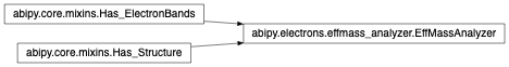
classmethod from_file(filepath)

Initialize the object from a netcdf file with an ebands object.

to_string(verbose)

Human-readable string with useful info such as band gaps, position of HOMO, LOMO…

Parameters

verbose – Verbosity level.

select_kpoint_band(kpoint, band, spin=0, etol_ev=0.001)

Construct line segments based on the k-point kpoint and the band index band. This is the most flexible interface and allows one to include extra bands by increasing the value of etol_ev.

Parameters

• kpoint – Fractional coordinates or abipy.core.kpoints.Kpoint object.

• band – Band index

• spin – Spin index.

• etol_ev – Include all bands at this k-point whose energy differ from the one at (kpoint, band) less that etol_ev in eV.

select_cbm(spin=0, etol_ev=0.001)

Select conduction band minimum.

select_vbm(spin=0, etol_ev=0.001)

Select valence band maximum.

select_band_edges(spin=0, etol_ev=0.001)

Select conduction band minimum and valence band maximum.

property ebands

abipy.electrons.ebands.ElectronBands object.

property structure

abipy.core.structure.Structure object.

summarize(acc=4)

plot_emass(acc=4, fontsize=6, colormap='viridis', **kwargs)

Plot electronic dispersion and quadratic curve based on the effective masses computed along each segment.

Parameters

• acc –

• fontsize – legend and title fontsize.

• colormap – matplotlib colormap

Keyword arguments controlling the display of the figure:

kwargs	Meaning
title	Title of the plot (Default: None).
show	True to show the figure (default: True).
savefig	“abc.png” or “abc.eps” to save the figure to a file.
size_kwargs	Dictionary with options passed to fig.set_size_inches e.g. size_kwargs=dict(w=3, h=4)
tight_layout	True to call fig.tight_layout (default: False)
ax_grid	True (False) to add (remove) grid from all axes in fig. Default: None i.e. fig is left unchanged.
ax_annotate	Add labels to subplots e.g. (a), (b). Default: False
fig_close	Close figure. Default: False.

plot_all_segments(ax=None, colormap='viridis', fontsize=8, **kwargs)

Parameters

• colormap – matplotlib colormap

• fontsize – legend and title fontsize.

Return: matplotlib.figure.Figure

Keyword arguments controlling the display of the figure:

kwargs	Meaning
title	Title of the plot (Default: None).
show	True to show the figure (default: True).
savefig	“abc.png” or “abc.eps” to save the figure to a file.
size_kwargs	Dictionary with options passed to fig.set_size_inches e.g. size_kwargs=dict(w=3, h=4)
tight_layout	True to call fig.tight_layout (default: False)
ax_grid	True (False) to add (remove) grid from all axes in fig. Default: None i.e. fig is left unchanged.
ax_annotate	Add labels to subplots e.g. (a), (b). Default: False
fig_close	Close figure. Default: False.

class abipy.electrons.effmass_analyzer.Segment(ik, spin, line, band_inds, ebands)

Bases: object

Z

Atomic number

to_string(verbose=0)

String representation.

get_fd_emass_d2(enes_kline, acc)

get_dataframe_with_accuracies(acc_list=(2, 4, 6, 8))

Build and return a pandas.DataFrame with effective masses computed with different accuracies (npts)

plot_emass(acc=4, ax=None, fontsize=8, colormap='viridis', **kwargs)

Parameters

• acc –

• ax – matplotlib.axes.Axes or None if a new figure should be created.

• fontsize – legend and title fontsize.

• colormap – matplotlib colormap

Return: matplotlib.figure.Figure

Keyword arguments controlling the display of the figure:

kwargs	Meaning
title	Title of the plot (Default: None).
show	True to show the figure (default: True).
savefig	“abc.png” or “abc.eps” to save the figure to a file.
size_kwargs	Dictionary with options passed to fig.set_size_inches e.g. size_kwargs=dict(w=3, h=4)
tight_layout	True to call fig.tight_layout (default: False)
ax_grid	True (False) to add (remove) grid from all axes in fig. Default: None i.e. fig is left unchanged.
ax_annotate	Add labels to subplots e.g. (a), (b). Default: False
fig_close	Close figure. Default: False.

fatbands Module

Classes for the analysis of electronic fatbands and projected DOSes.

abipy.electrons.fatbands.gaussians_dos(dos, mesh, width, values, energies, weights)

class abipy.electrons.fatbands.FatBandsFile(filepath)

Bases: abipy.core.mixins.AbinitNcFile, abipy.core.mixins.Has_Header, abipy.core.mixins.Has_Structure, abipy.core.mixins.Has_ElectronBands, abipy.core.mixins.NotebookWriter

Provides methods to analyze the data stored in the FATBANDS.nc file.

Usage example:

with abiopen("out_FATBANDS.nc") as fb:
    print(fb.structure)
    fb.plot_fatbands_lview()

Alternatively, one can use the abiopen.py script to open the file in an ipython notebook with:

abiopen.py out_FATBANDS.nc -nb

Inheritance Diagram

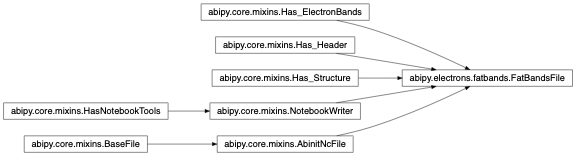
l2color = {0: 'red', 1: 'blue', 2: 'green', 3: 'yellow', 4: 'orange'}

l2tex = {0: '$l=s$', 1: '$l=p$', 2: '$l=d$', 3: '$l=f$', 4: '$l=g$'}

marker_spin = {0: '^', 1: 'v'}

marker_spin_plotly = {0: 5, 1: 6}

spin2tex = {0: '$\\sigma=\\uparrow$', 1: '$\\sigma=\\downarrow$'}

spinors2tex = {'down-down': '$\\downarrow,\\downarrow$', 'down-up': '$\\downarrow,\\uparrow$', 'sigma_x': '$\\sigma_{x}$', 'sigma_y': '$\\sigma_{y}$', 'sigma_z': '$\\sigma_{z}$', 'up-down': '$\\uparrow,\\downarrow$', 'up-up': '$\\uparrow,\\uparrow$'}

spinors2color = {'down-down': 'yellow', 'down-up': 'violet', 'sigma_x': 'green', 'sigma_y': 'blue', 'sigma_z': 'red', 'up-down': 'brown', 'up-up': 'black'}

alpha = 0.6

marker_size = 3.0

linewidth = 0.1

linecolor = 'grey'

classmethod from_file(filepath)

Initialize the object from a netcdf file

wal_sbk()

numpy.ndarray of shape [natom, mbesslang, nsppol, mband, nkpt] with the L-contributions. Present only if prtdos == 3.

walm_sbk()

numpy.ndarray of shape [natom, mbesslang**2, nsppol, mband, nkpt] with the LM-contribution. Present only if prtdos == 3 and prtdosm != 0

property ebands

abipy.electrons.ebands.ElectronBands object.

property structure

abipy.core.structure.Structure object.

params()

OrderedDict with parameters that might be subject to convergence studies.

close()

Called at the end of the with context manager.

to_string(verbose=0)

String representation.

get_wl_atom(iatom, spin=None, band=None)

Return the l-dependent DOS weights for atom index iatom. The weights are summed over m. If spin and band are not specified, the method returns the weights for all spin and bands else the contribution for (spin, band)

get_wl_symbol(symbol, spin=None, band=None)

Return the l-dependent DOS weights for a given type specified in terms of the chemical symbol symbol. The weights are summed over m and over all atoms of the same type. If spin and band are not specified, the method returns the weights for all spins and bands else the contribution for (spin, band).

get_w_symbol(symbol, spin=None, band=None)

Return the DOS weights for a given type specified in terms of the chemical symbol symbol. The weights are summed over m and lmax[symbol] and over all atoms of the same type. If spin and band are not specified, the method returns the weights for all spins and bands else the contribution for (spin, band).

get_spilling(spin=None, band=None)

Return the spilling parameter If spin and band are not specified, the method returns the spilling for all states as a [nsppol, mband, nkpt] numpy array else the spilling for (spin, band) with shape [nkpt].

eb_plotax_kwargs(spin)

Dictionary with the options passed to ebands.plot_ax when plotting a band line with spin index spin. Subclasses can redefine the implementation to customize the plots.

eb_plotly_kwargs(spin)

Dictionary with the options passed to ebands.plot_ax when plotting a band line with spin index spin. Subclasses can redefine the implementation to customize the plots.

plot_fatbands_siteview(e0='fermie', view='inequivalent', fact=1.0, fontsize=12, ylims=None, blist=None, **kwargs)

Plot fatbands for each atom in the unit cell. By default, only the inequivalent atoms are shown.

Parameters

• e0 – Option used to define the zero of energy in the band structure plot. Possible values: - fermie: shift all eigenvalues to have zero energy at the Fermi energy. - Number e.g e0 = 0.5: shift all eigenvalues to have zero energy at 0.5 eV - None: Don’t shift energies, equivalent to e0 = 0

• view – “inequivalent”, “all”

• fact – float used to scale the stripe size.

• fontsize – fontsize for titles and legend

• ylims – Set the data limits for the y-axis. Accept tuple e.g. (left, right) or scalar e.g. left. If left (right) is None, default values are used

• blist – List of band indices for the fatband plot. If None, all bands are included

Returns: matplotlib.figure.Figure

Keyword arguments controlling the display of the figure:

kwargs	Meaning
title	Title of the plot (Default: None).
show	True to show the figure (default: True).
savefig	“abc.png” or “abc.eps” to save the figure to a file.
size_kwargs	Dictionary with options passed to fig.set_size_inches e.g. size_kwargs=dict(w=3, h=4)
tight_layout	True to call fig.tight_layout (default: False)
ax_grid	True (False) to add (remove) grid from all axes in fig. Default: None i.e. fig is left unchanged.
ax_annotate	Add labels to subplots e.g. (a), (b). Default: False
fig_close	Close figure. Default: False.

plot_fatbands_lview(e0='fermie', fact=1.0, ax_mat=None, lmax=None, ylims=None, blist=None, fontsize=12, **kwargs)

Plot the electronic fatbands grouped by L with matplotlib.

Parameters

• e0 – Option used to define the zero of energy in the band structure plot. Possible values: - fermie: shift all eigenvalues to have zero energy at the Fermi energy. - Number e.g e0 = 0.5: shift all eigenvalues to have zero energy at 0.5 eV - None: Don’t shift energies, equivalent to e0 = 0

• fact – float used to scale the stripe size.

• ax_mat – Matrix of axes, if None a new figure is produced.

• lmax – Maximum L included in plot. None means full set available on file.

• ylims – Set the data limits for the y-axis. Accept tuple e.g. (left, right) or scalar e.g. left. If left (right) is None, default values are used

• blist – List of band indices for the fatband plot. If None, all bands are included

• fontsize – Legend fontsize.

Returns: matplotlib.figure.Figure

Keyword arguments controlling the display of the figure:

kwargs	Meaning
title	Title of the plot (Default: None).
show	True to show the figure (default: True).
savefig	“abc.png” or “abc.eps” to save the figure to a file.
size_kwargs	Dictionary with options passed to fig.set_size_inches e.g. size_kwargs=dict(w=3, h=4)
tight_layout	True to call fig.tight_layout (default: False)
ax_grid	True (False) to add (remove) grid from all axes in fig. Default: None i.e. fig is left unchanged.
ax_annotate	Add labels to subplots e.g. (a), (b). Default: False
fig_close	Close figure. Default: False.

plotly_fatbands_lview(e0='fermie', fact=1.0, fig=None, lmax=None, ylims=None, blist=None, fontsize=12, band_and_dos=0, **kwargs)

Plot the electronic fatbands grouped by L with plotly.

Parameters

• e0 – Option used to define the zero of energy in the band structure plot. Possible values: - fermie: shift all eigenvalues to have zero energy at the Fermi energy. - Number e.g e0 = 0.5: shift all eigenvalues to have zero energy at 0.5 eV - None: Don’t shift energies, equivalent to e0 = 0

• fact – float used to scale the stripe size.

• fig – The fig to plot on. None if a new figure should be created.

• lmax – Maximum L included in plot. None means full set available on file.

• ylims – Set the data limits for the y-axis. Accept tuple e.g. (left, right)

• blist – List of band indices for the fatband plot. If None, all bands are included

• fontsize – Legend and subtitle fontsize.

• band_and_dos – Define if both band and dos will be plotted on the same fig. If 0 (default), only plot band on the created figure (when fig==None); If 1, plot band on odd_col of fig

Returns: plotly.graph_objects.Figure

Keyword arguments controlling the display of the figure: ================ ==================================================================== kwargs Meaning ================ ==================================================================== title Title of the plot (Default: None). show True to show the figure (default: True). hovormode True to show the hover info (default: False) savefig “abc.png” , “abc.jpeg” or “abc.webp” to save the figure to a file. write_json Write plotly figure to write_json JSON file.

Inside jupyter-lab, one can right-click the write_json file from the file menu and open with “Plotly Editor”. Make some changes to the figure, then use the file menu to save the customized plotly plot. Requires jupyter labextension install jupyterlab-chart-editor. See https://github.com/plotly/jupyterlab-chart-editor

renderer (str or None (default None)) –

A string containing the names of one or more registered renderers (separated by ‘+’ characters) or None. If None, then the default renderers specified in plotly.io.renderers.default are used. See https://plotly.com/python-api-reference/generated/plotly.graph_objects.Figure.html

config (dict) A dict of parameters to configure the figure. The defaults are set in plotly.js. chart_studio True to push figure to chart_studio server. Requires authenticatios.

Default: False.

plot_fatbands_mview(iatom, e0='fermie', fact=1.0, lmax=None, ylims=None, blist=None, **kwargs)

Plot the electronic fatbands grouped by LM.

Parameters

• iatom – Index of the atom in the structure.

• e0 – Option used to define the zero of energy in the band structure plot. Possible values: - fermie: shift all eigenvalues to have zero energy at the Fermi energy. - Number e.g e0 = 0.5: shift all eigenvalues to have zero energy at 0.5 eV - None: Don’t shift energies, equivalent to e0 = 0

• fact – float used to scale the stripe size.

• lmax – Maximum L included in plot. None means full set available on file.

• ylims – Set the data limits for the y-axis. Accept tuple e.g. (left, right) or scalar e.g. left. If left (right) is None, default values are used

• blist – List of band indices for the fatband plot. If None, all bands are included

Returns: matplotlib.figure.Figure

Keyword arguments controlling the display of the figure:

kwargs	Meaning
title	Title of the plot (Default: None).
show	True to show the figure (default: True).
savefig	“abc.png” or “abc.eps” to save the figure to a file.
size_kwargs	Dictionary with options passed to fig.set_size_inches e.g. size_kwargs=dict(w=3, h=4)
tight_layout	True to call fig.tight_layout (default: False)
ax_grid	True (False) to add (remove) grid from all axes in fig. Default: None i.e. fig is left unchanged.
ax_annotate	Add labels to subplots e.g. (a), (b). Default: False
fig_close	Close figure. Default: False.

plot_fatbands_typeview(e0='fermie', fact=1.0, lmax=None, ax_mat=None, ylims=None, blist=None, fontsize=8, **kwargs)

Plot the electronic fatbands grouped by atomic type with matplotlib.

Parameters

• e0 – Option used to define the zero of energy in the band structure plot. Possible values: - fermie: shift all eigenvalues to have zero energy at the Fermi energy. - Number e.g e0 = 0.5: shift all eigenvalues to have zero energy at 0.5 eV - None: Don’t shift energies, equivalent to e0 = 0

• fact – float used to scale the stripe size.

• lmax – Maximum L included in plot. None means full set available on file.

• ax_mat – Matrix of axis. None if a new figure should be created.

• ylims – Set the data limits for the y-axis. Accept tuple e.g. (left, right) or scalar e.g. left. If left (right) is None, default values are used

• blist – List of band indices for the fatband plot. If None, all bands are included

• fontsize – Legend fontsize.

Returns: matplotlib.figure.Figure

Keyword arguments controlling the display of the figure:

kwargs	Meaning
title	Title of the plot (Default: None).
show	True to show the figure (default: True).
savefig	“abc.png” or “abc.eps” to save the figure to a file.
size_kwargs	Dictionary with options passed to fig.set_size_inches e.g. size_kwargs=dict(w=3, h=4)
tight_layout	True to call fig.tight_layout (default: False)
ax_grid	True (False) to add (remove) grid from all axes in fig. Default: None i.e. fig is left unchanged.
ax_annotate	Add labels to subplots e.g. (a), (b). Default: False
fig_close	Close figure. Default: False.

plotly_fatbands_typeview(e0='fermie', fact=1.0, lmax=None, fig=None, ylims=None, blist=None, fontsize=12, band_and_dos=0, **kwargs)

Plot the electronic fatbands grouped by atomic type with plotly.

Parameters

• e0 – Option used to define the zero of energy in the band structure plot. Possible values: - fermie: shift all eigenvalues to have zero energy at the Fermi energy. - Number e.g e0 = 0.5: shift all eigenvalues to have zero energy at 0.5 eV - None: Don’t shift energies, equivalent to e0 = 0

• fact – float used to scale the stripe size.

• lmax – Maximum L included in plot. None means full set available on file.

• fig – The fig to plot on. None if a new figure should be created.

• ylims – Set the data limits for the y-axis. Accept tuple e.g. (left, right)

• blist – List of band indices for the fatband plot. If None, all bands are included

• fontsize – Legend and subtitle fontsize.

• band_and_dos – Define if both band and dos will be plotted on the same fig. If 0(default), only plot band on the created figure (when fig==None); If 1, plot band on odd_col of fig

Returns: plotly.graph_objects.Figure

Keyword arguments controlling the display of the figure: ================ ==================================================================== kwargs Meaning ================ ==================================================================== title Title of the plot (Default: None). show True to show the figure (default: True). hovormode True to show the hover info (default: False) savefig “abc.png” , “abc.jpeg” or “abc.webp” to save the figure to a file. write_json Write plotly figure to write_json JSON file.

Inside jupyter-lab, one can right-click the write_json file from the file menu and open with “Plotly Editor”. Make some changes to the figure, then use the file menu to save the customized plotly plot. Requires jupyter labextension install jupyterlab-chart-editor. See https://github.com/plotly/jupyterlab-chart-editor

renderer (str or None (default None)) –

A string containing the names of one or more registered renderers (separated by ‘+’ characters) or None. If None, then the default renderers specified in plotly.io.renderers.default are used. See https://plotly.com/python-api-reference/generated/plotly.graph_objects.Figure.html

config (dict) A dict of parameters to configure the figure. The defaults are set in plotly.js. chart_studio True to push figure to chart_studio server. Requires authenticatios.

Default: False.

plot_spilling(e0='fermie', fact=1.0, ax_list=None, ylims=None, blist=None, **kwargs)

Plot the electronic fatbands

Parameters

• e0 – Option used to define the zero of energy in the band structure plot. Possible values: - fermie: shift all eigenvalues to have zero energy at the Fermi energy. - Number e.g e0 = 0.5: shift all eigenvalues to have zero energy at 0.5 eV - None: Don’t shift energies, equivalent to e0 = 0

• fact – float used to scale the stripe size.

• ax_list – List of matplotlib axes for plot. If None, new figure is produced

• ylims – Set the data limits for the y-axis. Accept tuple e.g. (left, right) or scalar e.g. left. If left (right) is None, default values are used

• blist – List of band indices for the fatband plot. If None, all bands are included

Returns: matplotlib.figure.Figure

Keyword arguments controlling the display of the figure:

kwargs	Meaning
title	Title of the plot (Default: None).
show	True to show the figure (default: True).
savefig	“abc.png” or “abc.eps” to save the figure to a file.
size_kwargs	Dictionary with options passed to fig.set_size_inches e.g. size_kwargs=dict(w=3, h=4)
tight_layout	True to call fig.tight_layout (default: False)
ax_grid	True (False) to add (remove) grid from all axes in fig. Default: None i.e. fig is left unchanged.
ax_annotate	Add labels to subplots e.g. (a), (b). Default: False
fig_close	Close figure. Default: False.

get_dos_integrator(method, step, width)

FatBandsFile can use differerent integrators that are cached in self._cached_dos_integrators

plot_pjdos_lview(e0='fermie', lmax=None, method='gaussian', step=0.1, width=0.2, stacked=True, combined_spins=True, ax_mat=None, exchange_xy=False, with_info=True, with_spin_sign=True, xlims=None, ylims=None, fontsize=8, **kwargs)

Plot the PJ-DOS on a linear mesh with matplotlib.

Parameters

• e0 – Option used to define the zero of energy in the band structure plot. Possible values: - fermie: shift all eigenvalues to have zero energy at the Fermi energy. - Number e.g e0 = 0.5: shift all eigenvalues to have zero energy at 0.5 eV - None: Don’t shift energies, equivalent to e0 = 0

• lmax – Maximum L included in plot. None means full set available on file.

• method – String defining the method for the computation of the DOS.

• step – Energy step (eV) of the linear mesh.

• width – Standard deviation (eV) of the gaussian.

• stacked – True if DOS partial contributions should be stacked on top of each other.

• combined_spins – Define how up/down DOS components should be plotted when nsppol==2. If True, up/down DOSes are plotted on the same figure (positive values for up, negative values for down component) If False, up/down components are plotted on different axes.

• ax_mat –

• exchange_xy – True if the dos should be plotted on the x axis instead of y.

• xlims – Set the data limits for the x-axis. Accept tuple e.g. (left, right) or scalar e.g. left. If left (right) is None, default values are used

• ylims – Same meaning as xlims but for the y-axis

• fontsize – Legend and subtitle fontsize

Returns: matplotlib.figure.Figure

Keyword arguments controlling the display of the figure:

kwargs	Meaning
title	Title of the plot (Default: None).
show	True to show the figure (default: True).
savefig	“abc.png” or “abc.eps” to save the figure to a file.
size_kwargs	Dictionary with options passed to fig.set_size_inches e.g. size_kwargs=dict(w=3, h=4)
tight_layout	True to call fig.tight_layout (default: False)
ax_grid	True (False) to add (remove) grid from all axes in fig. Default: None i.e. fig is left unchanged.
ax_annotate	Add labels to subplots e.g. (a), (b). Default: False
fig_close	Close figure. Default: False.

plotly_pjdos_lview(e0='fermie', lmax=None, method='gaussian', step=0.1, width=0.2, stacked=True, combined_spins=True, fig=None, exchange_xy=False, with_info=True, with_spin_sign=True, xlims=None, ylims=None, fontsize=12, band_and_dos=0, **kwargs)

Plot the PJ-DOS on a linear mesh with plotly.

Parameters

• e0 – Option used to define the zero of energy in the band structure plot. Possible values: - fermie: shift all eigenvalues to have zero energy at the Fermi energy. - Number e.g e0 = 0.5: shift all eigenvalues to have zero energy at 0.5 eV - None: Don’t shift energies, equivalent to e0 = 0

• lmax – Maximum L included in plot. None means full set available on file.

• method – String defining the method for the computation of the DOS.

• step – Energy step (eV) of the linear mesh.

• width – Standard deviation (eV) of the gaussian.

• stacked – True if DOS partial contributions should be stacked on top of each other.

• combined_spins – Define how up/down DOS components should be plotted when nsppol==2. If True, up/down DOSes are plotted on the same figure (positive values for up, negative values for down component) If False, up/down components are plotted on different axes.

• fig – The fig to plot on. None if a new figure should be created.

• exchange_xy – True if the dos should be plotted on the x axis instead of y.

• xlims – Set the data limits for the x-axis. Accept tuple e.g. (left, right)

• ylims – Same meaning as xlims but for the y-axis

• fontsize – Legend and subtitle fontsize.

• band_and_dos – Define if both band and dos will be plotted on the same fig. If 0(default), only plot dos on the created figure (when fig==None); If 1, plot dos on even_col of fig

Returns: plotly.graph_objects.Figure

Keyword arguments controlling the display of the figure: ================ ==================================================================== kwargs Meaning ================ ==================================================================== title Title of the plot (Default: None). show True to show the figure (default: True). hovormode True to show the hover info (default: False) savefig “abc.png” , “abc.jpeg” or “abc.webp” to save the figure to a file. write_json Write plotly figure to write_json JSON file.

Inside jupyter-lab, one can right-click the write_json file from the file menu and open with “Plotly Editor”. Make some changes to the figure, then use the file menu to save the customized plotly plot. Requires jupyter labextension install jupyterlab-chart-editor. See https://github.com/plotly/jupyterlab-chart-editor

renderer (str or None (default None)) –

A string containing the names of one or more registered renderers (separated by ‘+’ characters) or None. If None, then the default renderers specified in plotly.io.renderers.default are used. See https://plotly.com/python-api-reference/generated/plotly.graph_objects.Figure.html

config (dict) A dict of parameters to configure the figure. The defaults are set in plotly.js. chart_studio True to push figure to chart_studio server. Requires authenticatios.

Default: False.

plot_pjdos_typeview(e0='fermie', lmax=None, method='gaussian', step=0.1, width=0.2, stacked=True, combined_spins=True, ax_mat=None, exchange_xy=False, with_info=True, with_spin_sign=True, xlims=None, ylims=None, fontsize=8, **kwargs)

Plot the PJ-DOS on a linear mesh with matplotlib.

Parameters

• e0 – Option used to define the zero of energy in the band structure plot. Possible values: - fermie: shift all eigenvalues to have zero energy at the Fermi energy. - Number e.g e0 = 0.5: shift all eigenvalues to have zero energy at 0.5 eV - None: Don’t shift energies, equivalent to e0 = 0

• lmax – Maximum L included in plot. None means full set available on file.

• method – String defining the method for the computation of the DOS.

• step – Energy step (eV) of the linear mesh.

• width – Standard deviation (eV) of the gaussian.

• stacked – True if DOS partial contributions should be stacked on top of each other.

• combined_spins – Define how up/down DOS components should be plotted when nsppol==2. If True, up/down DOSes are plotted on the same figure (positive values for up, negative values for down component) If False, up/down components are plotted on different axes.

• ax_mat –

• exchange_xy – True if the dos should be plotted on the x axis instead of y.

• xlims – Set the data limits for the x-axis. Accept tuple e.g. (left, right) or scalar e.g. left. If left (right) is None, default values are used

• ylims – Same meaning as xlims but for the y-axis

• fontsize – Legend and subtitle fontsize.

Returns: matplotlib.figure.Figure

Keyword arguments controlling the display of the figure:

kwargs	Meaning
title	Title of the plot (Default: None).
show	True to show the figure (default: True).
savefig	“abc.png” or “abc.eps” to save the figure to a file.
size_kwargs	Dictionary with options passed to fig.set_size_inches e.g. size_kwargs=dict(w=3, h=4)
tight_layout	True to call fig.tight_layout (default: False)
ax_grid	True (False) to add (remove) grid from all axes in fig. Default: None i.e. fig is left unchanged.
ax_annotate	Add labels to subplots e.g. (a), (b). Default: False
fig_close	Close figure. Default: False.

plotly_pjdos_typeview(e0='fermie', lmax=None, method='gaussian', step=0.1, width=0.2, stacked=True, combined_spins=True, fig=None, exchange_xy=False, with_info=True, with_spin_sign=True, xlims=None, ylims=None, fontsize=12, band_and_dos=0, **kwargs)

Plot the PJ-DOS on a linear mesh with plotly.

Parameters

• e0 – Option used to define the zero of energy in the band structure plot. Possible values: - fermie: shift all eigenvalues to have zero energy at the Fermi energy. - Number e.g e0 = 0.5: shift all eigenvalues to have zero energy at 0.5 eV - None: Don’t shift energies, equivalent to e0 = 0

• lmax – Maximum L included in plot. None means full set available on file.

• method – String defining the method for the computation of the DOS.

• step – Energy step (eV) of the linear mesh.

• width – Standard deviation (eV) of the gaussian.

• stacked – True if DOS partial contributions should be stacked on top of each other.

• combined_spins – Define how up/down DOS components should be plotted when nsppol==2. If True, up/down DOSes are plotted on the same figure (positive values for up, negative values for down component) If False, up/down components are plotted on different axes.

• fig – The fig to plot on. None if a new figure should be created.

• exchange_xy – True if the dos should be plotted on the x axis instead of y.

• xlims – Set the data limits for the x-axis. Accept tuple e.g. (left, right)

• ylims – Same meaning as xlims but for the y-axis

• fontsize – Legend and subtitle fontsize.

• band_and_dos – Define if both band and dos will be plotted on the same fig. If 0(default), only plot dos on the created figure (when fig==None); If 1, plot dos on even_col of fig

Returns: plotly.graph_objects.Figure

Keyword arguments controlling the display of the figure: ================ ==================================================================== kwargs Meaning ================ ==================================================================== title Title of the plot (Default: None). show True to show the figure (default: True). hovormode True to show the hover info (default: False) savefig “abc.png” , “abc.jpeg” or “abc.webp” to save the figure to a file. write_json Write plotly figure to write_json JSON file.

Inside jupyter-lab, one can right-click the write_json file from the file menu and open with “Plotly Editor”. Make some changes to the figure, then use the file menu to save the customized plotly plot. Requires jupyter labextension install jupyterlab-chart-editor. See https://github.com/plotly/jupyterlab-chart-editor

renderer (str or None (default None)) –

A string containing the names of one or more registered renderers (separated by ‘+’ characters) or None. If None, then the default renderers specified in plotly.io.renderers.default are used. See https://plotly.com/python-api-reference/generated/plotly.graph_objects.Figure.html

config (dict) A dict of parameters to configure the figure. The defaults are set in plotly.js. chart_studio True to push figure to chart_studio server. Requires authenticatios.

Default: False.

plot_fatbands_with_pjdos(e0='fermie', fact=1.0, lmax=None, blist=None, view='type', pjdosfile=None, edos_kwargs=None, stacked=True, width_ratios=(2, 1), fontsize=8, ylims=None, **kwargs)

Compute the fatbands and the PJDOS on the same figure with matplotlib, a.k.a the Sistine Chapel.

Parameters

• e0 – Option used to define the zero of energy in the band structure plot. Possible values: - fermie: shift all eigenvalues to have zero energy at the Fermi energy. - Number e.g e0 = 0.5: shift all eigenvalues to have zero energy at 0.5 eV - None: Don’t shift energies, equivalent to e0 = 0

• fact – float used to scale the stripe size.

• lmax – Maximum L included in plot. None means full set available on file.

• blist – List of band indices for the fatband plot. If None, all bands are included

• pjdosfile – FATBANDS file used to compute the PJDOS. If None, the PJDOS is taken from self.

• edos_kwargs –

• stacked – True if DOS partial contributions should be stacked on top of each other.

• width_ratios – Defines the ratio between the band structure plot and the dos plot.

• fontsize – Legend fontsize.

• ylims – Set the data limits for the y-axis. Accept tuple e.g. (left, right) or scalar e.g. left. If left (right) is None, default values are used

Returns: matplotlib.figure.Figure

Keyword arguments controlling the display of the figure:

kwargs	Meaning
title	Title of the plot (Default: None).
show	True to show the figure (default: True).
savefig	“abc.png” or “abc.eps” to save the figure to a file.
size_kwargs	Dictionary with options passed to fig.set_size_inches e.g. size_kwargs=dict(w=3, h=4)
tight_layout	True to call fig.tight_layout (default: False)
ax_grid	True (False) to add (remove) grid from all axes in fig. Default: None i.e. fig is left unchanged.
ax_annotate	Add labels to subplots e.g. (a), (b). Default: False
fig_close	Close figure. Default: False.

plotly_fatbands_with_pjdos(e0='fermie', fact=1.0, lmax=None, blist=None, view='type', pjdosfile=None, edos_kwargs=None, stacked=True, width_ratios=(2, 1), fontsize=12, ylims=None, **kwargs)

Compute the fatbands and the PJDOS on the same figure with plotly, a.k.a the Sistine Chapel.

Parameters

• e0 – Option used to define the zero of energy in the band structure plot. Possible values: - fermie: shift all eigenvalues to have zero energy at the Fermi energy. - Number e.g e0 = 0.5: shift all eigenvalues to have zero energy at 0.5 eV - None: Don’t shift energies, equivalent to e0 = 0

• fact – float used to scale the stripe size.

• lmax – Maximum L included in plot. None means full set available on file.

• blist – List of band indices for the fatband plot. If None, all bands are included

• pjdosfile – FATBANDS file used to compute the PJDOS. If None, the PJDOS is taken from self.

• edos_kwargs –

• stacked – True if DOS partial contributions should be stacked on top of each other.

• width_ratios – Defines the ratio between the band structure plot and the dos plot.

• fontsize – Legend and subtitle fontsize.

• ylims – Set the data limits for the y-axis. Accept tuple e.g. (left, right)

Returns: plotly.graph_objects.Figure

Keyword arguments controlling the display of the figure: ================ ==================================================================== kwargs Meaning ================ ==================================================================== title Title of the plot (Default: None). show True to show the figure (default: True). hovormode True to show the hover info (default: False) savefig “abc.png” , “abc.jpeg” or “abc.webp” to save the figure to a file. write_json Write plotly figure to write_json JSON file.

Inside jupyter-lab, one can right-click the write_json file from the file menu and open with “Plotly Editor”. Make some changes to the figure, then use the file menu to save the customized plotly plot. Requires jupyter labextension install jupyterlab-chart-editor. See https://github.com/plotly/jupyterlab-chart-editor

renderer (str or None (default None)) –

A string containing the names of one or more registered renderers (separated by ‘+’ characters) or None. If None, then the default renderers specified in plotly.io.renderers.default are used. See https://plotly.com/python-api-reference/generated/plotly.graph_objects.Figure.html

config (dict) A dict of parameters to configure the figure. The defaults are set in plotly.js. chart_studio True to push figure to chart_studio server. Requires authenticatios.

Default: False.

plot_pawdos_terms(lmax=None, method='gaussian', step=0.1, width=0.2, xlims=None, *kwargs)

Plot …

Parameters

• lmax – Maximum L included in plot. None means full set available on file.

• method – String defining the method for the computation of the DOS.

• step – Energy step (eV) of the linear mesh.

• width – Standard deviation (eV) of the gaussian.

• xlims – Set the data limits for the x-axis. Accept tuple e.g. (left, right) or scalar e.g. left. If left (right) is None, default values are used

Returns: matplotlib.figure.Figure

Keyword arguments controlling the display of the figure:

kwargs	Meaning
title	Title of the plot (Default: None).
show	True to show the figure (default: True).
savefig	“abc.png” or “abc.eps” to save the figure to a file.
size_kwargs	Dictionary with options passed to fig.set_size_inches e.g. size_kwargs=dict(w=3, h=4)
tight_layout	True to call fig.tight_layout (default: False)
ax_grid	True (False) to add (remove) grid from all axes in fig. Default: None i.e. fig is left unchanged.
ax_annotate	Add labels to subplots e.g. (a), (b). Default: False
fig_close	Close figure. Default: False.

yield_figs(**kwargs)

This function generates a predefined list of matplotlib figures with minimal input from the user. Used in abiview.py to get a quick look at the results.

yield_plotly_figs(**kwargs)

This function generates a predefined list of plotly figures with minimal input from the user.

get_panel(**kwargs)

Build panel with widgets to interact with the abipy.electrons.fatbands.FatBandsFile either in a notebook or in panel app.

write_notebook(nbpath=None)

Write a jupyter notebook to nbpath. If nbpath is None, a temporay file in the current working directory is created. Return path to the notebook.

fold2bloch Module

Fold2Bloch netcdf file.

class abipy.electrons.fold2bloch.Fold2BlochNcfile(filepath)

Bases: abipy.core.mixins.AbinitNcFile, abipy.core.mixins.Has_Header, abipy.core.mixins.Has_Structure, abipy.core.mixins.Has_ElectronBands, abipy.core.mixins.NotebookWriter

Netcdf file with output data produced by Fold2Bloch.

Usage example:

with Fold2BlochNcfile("foo_FOLD2BLOCH.nc") as fb:
    fb.plot_unfolded()

Inheritance Diagram

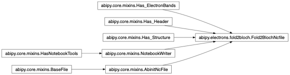
classmethod from_wfkpath(wfkpath, folds, workdir=None, manager=None, mpi_procs=1, verbose=0)

Run fold2bloch in workdir.

Parameters

• wfkpath –

• folds –

• workdir – Working directory of the fake task used to compute the ibz. Use None for temporary dir.

• manager – TaskManager of the task. If None, the manager is initialized from the config file.

• mpi_procs – Number of MPI processors to use.

• verbose – Verbosity level.

to_string(verbose=0)

String representation.

property ebands

abipy.electrons.ebands.ElectronBands object with folded band energies.

property structure

abipy.core.structure.Structure object defining the supercell.

close()

Close the file.

params()

OrderedDict with parameters that might be subject to convergence studies.

uf_eigens()

[nsppol, nk_unfolded, nband] numpy.ndarray with unfolded eigenvalues in eV.

uf_weights()

[nss, nk_unfolded, nband] array with spectral weights. nss = max(nspinor, nsppol).

get_spectral_functions(step=0.01, width=0.02)

Parameters

• step – Energy step (eV) of the linear mesh.

• width – Standard deviation (eV) of the gaussian.

Returns

mesh, sfw, int_sfw

plot_unfolded(kbounds, klabels, ylims=None, dist_tol=1e-12, verbose=0, colormap='afmhot', facecolor='black', ax=None, fontsize=12, **kwargs)

Plot unfolded band structure with spectral weights.

Parameters

• klabels – dictionary whose keys are tuple with the reduced coordinates of the k-points. The values are the labels. e.g. klabels = {(0.0,0.0,0.0): "$\Gamma$", (0.5,0,0): "L"}.

• ylims – Set the data limits for the y-axis. Accept tuple e.g. (left, right) or scalar e.g. left. If left (right) is None, default values are used

• dist_tol – A point is considered to be on the path if its distance from the line is less than dist_tol.

• verbose – Verbosity level.

• colormap – Have a look at the colormaps here and decide which one you like: http://matplotlib.sourceforge.net/examples/pylab_examples/show_colormaps.html

• facecolor –

• ax – matplotlib.axes.Axes or None if a new figure should be created.

• fontsize – Legend and title fontsize.

Returns: matplotlib.figure.Figure

Keyword arguments controlling the display of the figure:

kwargs	Meaning
title	Title of the plot (Default: None).
show	True to show the figure (default: True).
savefig	“abc.png” or “abc.eps” to save the figure to a file.
size_kwargs	Dictionary with options passed to fig.set_size_inches e.g. size_kwargs=dict(w=3, h=4)
tight_layout	True to call fig.tight_layout (default: False)
ax_grid	True (False) to add (remove) grid from all axes in fig. Default: None i.e. fig is left unchanged.
ax_annotate	Add labels to subplots e.g. (a), (b). Default: False
fig_close	Close figure. Default: False.

yield_figs(**kwargs)

This function generates a predefined list of matplotlib figures with minimal input from the user.

write_notebook(nbpath=None)

Write a jupyter notebook to nbpath. If nbpath is None, a temporay file in the current working directory is created. Return path to the notebook.

gsr Module

Interface to the GSR.nc file storing the Ground-state results and the electron band structure.

class abipy.electrons.gsr.GsrFile(filepath)

Bases: abipy.core.mixins.AbinitNcFile, abipy.core.mixins.Has_Header, abipy.core.mixins.Has_Structure, abipy.core.mixins.Has_ElectronBands, abipy.core.mixins.NotebookWriter

File containing the results of a ground-state calculation.

Usage example:

with GsrFile("foo_GSR.nc") as gsr:
    print("energy: ", gsr.energy)
    gsr.ebands.plot()

Inheritance Diagram

classmethod from_file(filepath)

Initialize the object from a netcdf file.

to_string(verbose=0)

String representation.

property ebands

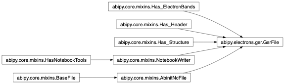
abipy.electrons.ebands.ElectronBands object.

is_scf_run()

True if the GSR has been produced by a SCF run.

ecut()

Cutoff energy in Hartree (Abinit input variable)

pawecutdg()

Cutoff energy in Hartree for the PAW double grid (Abinit input variable)

property structure

abipy.core.structure.Structure object.

energy()

Total energy in eV.

energy_per_atom()

Total energy / number_of_atoms (eV units)

cart_forces()

Cartesian forces in eV / Ang

max_force()

Max cart force in eV / Ang

force_stats(**kwargs)

Return a string with information on the forces.

cart_stress_tensor()

Stress tensor in GPa.

pressure()

Pressure in GPa.

residm()

Maximum of the residuals

xc()

XcFunc object with info on the exchange-correlation functional. Use libxc convention [Marques2012].

energy_terms()

EnergyTerms with the different contributions to the total energy in eV.

params()

OrderedDict with parameters that might be subject to convergence studies.

close()

Close the file.

as_dict()

get_computed_entry(inc_structure=True, parameters=None, data=None)

Returns a pymatgen ComputedStructureEntry from the GSR file. Same API as the one used in vasp_output.get_computed_entry.

Parameters

• inc_structure (bool) – Set to True if you want ComputedStructureEntries to be returned instead of ComputedEntries.

• parameters (list) – Input parameters to include. It has to be one of the properties supported by the GSR object. If parameters is None, a default set of parameters that are necessary for typical post-processing will be set.

• data (list) – Output data to include. Has to be one of the properties supported by the GSR object.

Returns

ComputedStructureEntry/ComputedEntry

get_panel(**kwargs)

Build panel with widgets to interact with the abipy.electrons.gsr.GsrFile either in a notebook or in panel app.

yield_figs(**kwargs)

This function generates a predefined list of matplotlib figures with minimal input from the user.

yield_plotly_figs(**kwargs)

This function generates a predefined list of plotly figures with minimal input from the user.

write_notebook(nbpath=None)

Write a jupyter notebook to nbpath. If nbpath is None, a temporay file in the current working directory is created. Return path to the notebook.

gw Module

Classes for the analysis of GW calculations.

class abipy.electrons.gw.QPState(spin, kpoint, band, e0, qpe, qpe_diago, vxcme, sigxme, sigcmee0, vUme, ze0)

Bases: abipy.electrons.gw.QPState

Quasi-particle result for given (spin, kpoint, band).

Note

Energies are in eV.

property qpeme0

E_QP - E_0

property re_qpe

Real part of the QP energy.

property imag_qpe

Imaginay part of the QP energy.

property skb

Tuple with (spin, kpoint, band)

copy()

Return Shallow copy.

classmethod get_fields(exclude=())

as_dict(**kwargs)

Convert self into a dictionary.

to_strdict(fmt=None)

Ordered dictionary mapping fields –> strings.

property tips

Bound method of self that returns a dictionary with the description of the fields.

classmethod TIPS()

Class method that returns a dictionary with the description of the fields. The string are extracted from the class doc string.

classmethod get_fields_for_plot(with_fields, exclude_fields)

Return list of QPState fields to plot from input arguments.

class abipy.electrons.gw.SigresFile(filepath)

Bases: abipy.core.mixins.AbinitNcFile, abipy.core.mixins.Has_Structure, abipy.core.mixins.Has_ElectronBands, abipy.core.mixins.NotebookWriter

Container storing the GW results reported in the SIGRES.nc file.

Usage example:

sigres = SigresFile("foo_SIGRES.nc")
sigres.plot_qps_vs_e0()

Inheritance Diagram

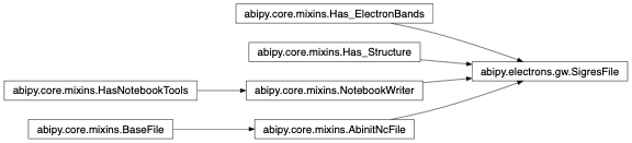
marker_spin = {0: '^', 1: 'v'}

color_spin = {0: 'k', 1: 'r'}

classmethod from_file(filepath)

Initialize an instance from file.

property sigma_kpoints

The K-points where QP corrections have been calculated.

get_marker(qpattr)

Return Marker object associated to the QP attribute qpattr. Used to prepare plots of KS bands with markers.

params()

OrderedDict with parameters that might be subject to convergence studies e.g ecuteps

close()

Close the netcdf file.

to_string(verbose=0)

String representation with verbosity level verbose.

property structure

abipy.core.structure.Structure object.

property ebands

abipy.electrons.ebands.ElectronBands with the KS energies.

property has_spectral_function

True if file contains spectral function data.

qplist_spin()

Tuple of QPList objects indexed by spin.

get_qplist(spin, kpoint, ignore_imag=False)

Return :class`QPList` for the given (spin, kpoint)

get_qpcorr(spin, kpoint, band, ignore_imag=False)

Returns the QPState object for the given (s, k, b)

qpgaps()

numpy.ndarray of shape [nsppol, nkibz] with the QP direct gaps in eV.

get_qpgap(spin, kpoint, with_ksgap=False)

Return the QP gap in eV at the given (spin, kpoint)

read_sigee_skb(spin, kpoint, band)

” Read self-energy(w) for (spin, kpoint, band) Return: SelfEnergy object

print_qps(precision=3, ignore_imag=True, file=<_io.TextIOWrapper name='<stdout>' mode='w' encoding='utf-8'>)

Print QP results to stream file.

Parameters

• precision – Number of significant digits.

• ignore_imag – True if imaginary part should be ignored.

• file – Output stream.

get_points_from_ebands(ebands_kpath, dist_tol=1e-12, size=24, verbose=0)

Generate object storing the QP energies lying on the k-path used by ebands_kpath. Mainly used to plot the QP energies in ebands.plot when the QP energies are interpolated with the SKW method.

Parameters

• ebands_kpath – abipy.electrons.ebands.ElectronBands object with the QP energies along an arbitrary k-path.

• dist_tol – A point is considered to be on the path if its distance from the line is less than dist_tol.

• size – The marker size in points**2

• verbose – Verbosity level

Return:

Example:

r = sigres.interpolate(lpratio=5,
                       ks_ebands_kpath=ks_ebands_kpath,
                       ks_ebands_kmesh=ks_ebands_kmesh
                       )
points = sigres.get_points_from_ebands(r.qp_ebands_kpath, size=24)
r.qp_ebands_kpath.plot(points=points)

plot_qpgaps(ax=None, plot_qpmks=True, fontsize=8, **kwargs)

Plot the KS and the QP direct gaps for all the k-points and spins available on file.

Parameters

• ax – matplotlib.axes.Axes or None if a new figure should be created.

• plot_qpmks – If False, plot QP_gap, KS_gap else (QP_gap - KS_gap)

• fontsize – legend and title fontsize.

• kwargs – Passed to ax.plot method except for marker.

Returns: matplotlib.figure.Figure

Keyword arguments controlling the display of the figure:

kwargs	Meaning
title	Title of the plot (Default: None).
show	True to show the figure (default: True).
savefig	“abc.png” or “abc.eps” to save the figure to a file.
size_kwargs	Dictionary with options passed to fig.set_size_inches e.g. size_kwargs=dict(w=3, h=4)
tight_layout	True to call fig.tight_layout (default: False)
ax_grid	True (False) to add (remove) grid from all axes in fig. Default: None i.e. fig is left unchanged.
ax_annotate	Add labels to subplots e.g. (a), (b). Default: False
fig_close	Close figure. Default: False.

plot_qps_vs_e0(with_fields='all', exclude_fields=None, e0='fermie', xlims=None, sharey=False, ax_list=None, fontsize=8, **kwargs)

Plot QP result in SIGRES file as function of the KS energy.

Parameters

• with_fields – The names of the qp attributes to plot as function of eKS. Accepts: List of strings or string with tokens separated by blanks. See QPState for the list of available fields.

• exclude_fields – Similar to with_fields but excludes fields

• e0 – Option used to define the zero of energy in the band structure plot. Possible values: - fermie: shift all eigenvalues to have zero energy at the Fermi energy (self.fermie). - Number e.g e0=0.5: shift all eigenvalues to have zero energy at 0.5 eV - None: Don’t shift energies, equivalent to e0=0

• ax_list – List of matplotlib.axes.Axes for plot. If None, new figure is produced.

• xlims – Set the data limits for the x-axis. Accept tuple e.g. (left, right) or scalar e.g. left. If left (right) is None, default values are used.

• sharey – True if y-axis should be shared.

• fontsize – Legend and title fontsize.

Returns: matplotlib.figure.Figure

Keyword arguments controlling the display of the figure:

kwargs	Meaning
title	Title of the plot (Default: None).
show	True to show the figure (default: True).
savefig	“abc.png” or “abc.eps” to save the figure to a file.
size_kwargs	Dictionary with options passed to fig.set_size_inches e.g. size_kwargs=dict(w=3, h=4)
tight_layout	True to call fig.tight_layout (default: False)
ax_grid	True (False) to add (remove) grid from all axes in fig. Default: None i.e. fig is left unchanged.
ax_annotate	Add labels to subplots e.g. (a), (b). Default: False
fig_close	Close figure. Default: False.

plot_spectral_functions(include_bands=None, fontsize=8, **kwargs)

Plot the spectral function for all k-points, bands and spins available in the SIGRES file.

Parameters

• include_bands – List of bands to include. Nonee means all.

• fontsize – Legend and title fontsize.

Returns: matplotlib.figure.Figure

Keyword arguments controlling the display of the figure:

kwargs	Meaning
title	Title of the plot (Default: None).
show	True to show the figure (default: True).
savefig	“abc.png” or “abc.eps” to save the figure to a file.
size_kwargs	Dictionary with options passed to fig.set_size_inches e.g. size_kwargs=dict(w=3, h=4)
tight_layout	True to call fig.tight_layout (default: False)
ax_grid	True (False) to add (remove) grid from all axes in fig. Default: None i.e. fig is left unchanged.
ax_annotate	Add labels to subplots e.g. (a), (b). Default: False
fig_close	Close figure. Default: False.

plot_eigvec_qp(spin=0, kpoint=None, band=None, **kwargs)

Parameters

• spin – Spin index

• kpoint – K-point in self-energy. Accepts abipy.core.kpoints.Kpoint, vector or index. If None, all k-points for the given spin are shown.

• band – band index. If None all bands are displayed else only <KS_b|QP_{b’}> for the given b.

• kwargs – Passed to plot method of ArrayPlotter.

Returns: matplotlib.figure.Figure

Keyword arguments controlling the display of the figure:

kwargs	Meaning
title	Title of the plot (Default: None).
show	True to show the figure (default: True).
savefig	“abc.png” or “abc.eps” to save the figure to a file.
size_kwargs	Dictionary with options passed to fig.set_size_inches e.g. size_kwargs=dict(w=3, h=4)
tight_layout	True to call fig.tight_layout (default: False)
ax_grid	True (False) to add (remove) grid from all axes in fig. Default: None i.e. fig is left unchanged.
ax_annotate	Add labels to subplots e.g. (a), (b). Default: False
fig_close	Close figure. Default: False.

plot_qpbands_ibz(e0='fermie', colormap='jet', ylims=None, fontsize=8, **kwargs)

Plot the KS band structure in the IBZ with the QP energies.

Parameters

• e0 – Option used to define the zero of energy in the band structure plot.

• colormap – matplotlib color map.

• ylims – Set the data limits for the y-axis. Accept tuple e.g. (left, right) or scalar e.g. left. If left (right) is None, default values are used.

• fontsize – Legend and title fontsize.

Returns: matplotlib.figure.Figure

Keyword arguments controlling the display of the figure:

kwargs	Meaning
title	Title of the plot (Default: None).
show	True to show the figure (default: True).
savefig	“abc.png” or “abc.eps” to save the figure to a file.
size_kwargs	Dictionary with options passed to fig.set_size_inches e.g. size_kwargs=dict(w=3, h=4)
tight_layout	True to call fig.tight_layout (default: False)
ax_grid	True (False) to add (remove) grid from all axes in fig. Default: None i.e. fig is left unchanged.
ax_annotate	Add labels to subplots e.g. (a), (b). Default: False
fig_close	Close figure. Default: False.

plot_ksbands_with_qpmarkers(qpattr='qpeme0', e0='fermie', fact=1000, ax=None, **kwargs)

Plot the KS energies as function of k-points and add markers whose size is proportional to the QPState attribute qpattr

Parameters

• qpattr – Name of the QP attribute to plot. See QPState.

• e0 – Option used to define the zero of energy in the band structure plot. Possible values: - fermie: shift all eigenvalues to have zero energy at the Fermi energy (self.fermie). - Number e.g e0 = 0.5: shift all eigenvalues to have zero energy at 0.5 eV - None: Don’t shift energies, equivalent to e0 = 0

• fact – Markers are multiplied by this factor.

• ax – matplotlib.axes.Axes or None if a new figure should be created.

Returns: matplotlib.figure.Figure

Keyword arguments controlling the display of the figure:

kwargs	Meaning
title	Title of the plot (Default: None).
show	True to show the figure (default: True).
savefig	“abc.png” or “abc.eps” to save the figure to a file.
size_kwargs	Dictionary with options passed to fig.set_size_inches e.g. size_kwargs=dict(w=3, h=4)
tight_layout	True to call fig.tight_layout (default: False)
ax_grid	True (False) to add (remove) grid from all axes in fig. Default: None i.e. fig is left unchanged.
ax_annotate	Add labels to subplots e.g. (a), (b). Default: False
fig_close	Close figure. Default: False.

get_dataframe(ignore_imag=False)

Returns pandas.DataFrame with QP results for all k-points included in the GW calculation

Parameters

ignore_imag – Only real part is returned if ignore_imag.

to_dataframe(ignore_imag=False)

Returns pandas.DataFrame with QP results for all k-points included in the GW calculation

Parameters

ignore_imag – Only real part is returned if ignore_imag.

get_dataframe_sk(spin, kpoint, index=None, ignore_imag=False, with_params=True)

Returns pandas.DataFrame with QP results for the given (spin, k-point).

Parameters

• ignore_imag – Only real part is returned if ignore_imag.

• with_params – True to include convergence paramenters.

interpolate(lpratio=5, ks_ebands_kpath=None, ks_ebands_kmesh=None, ks_degatol=0.0001, vertices_names=None, line_density=20, filter_params=None, only_corrections=False, verbose=0)

Interpolate the GW corrections in k-space on a k-path and, optionally, on a k-mesh.

Parameters

• lpratio – Ratio between the number of star functions and the number of ab-initio k-points. The default should be OK in many systems, larger values may be required for accurate derivatives.

• ks_ebands_kpath – KS abipy.electrons.ebands.ElectronBands on a k-path. If present, the routine interpolates the QP corrections and apply them on top of the KS band structure This is the recommended option because QP corrections are usually smoother than the QP energies and therefore easier to interpolate. If None, the QP energies are interpolated along the path defined by vertices_names and line_density.

• ks_ebands_kmesh – KS abipy.electrons.ebands.ElectronBands on a homogeneous k-mesh. If present, the routine interpolates the corrections on the k-mesh (used to compute QP the DOS)

• ks_degatol – Energy tolerance in eV. Used when either ks_ebands_kpath or ks_ebands_kmesh are given. KS energies are assumed to be degenerate if they differ by less than this value. The interpolator may break band degeneracies (the error is usually smaller if QP corrections are interpolated instead of QP energies). This problem can be partly solved by averaging the interpolated values over the set of KS degenerate states. A negative value disables this ad-hoc symmetrization.

• vertices_names – Used to specify the k-path for the interpolated QP band structure when ks_ebands_kpath is None. It’s a list of tuple, each tuple is of the form (kfrac_coords, kname) where kfrac_coords are the reduced coordinates of the k-point and kname is a string with the name of the k-point. Each point represents a vertex of the k-path. line_density defines the density of the sampling. If None, the k-path is automatically generated according to the point group of the system.

• line_density – Number of points in the smallest segment of the k-path. Used with vertices_names.

• filter_params – TO BE DESCRIBED

• only_corrections – If True, the output contains the interpolated QP corrections instead of the QP energies. Available only if ks_ebands_kpath and/or ks_ebands_kmesh are used.

• verbose – Verbosity level

Returns

namedtuple with the following attributes:

* qp_ebands_kpath: |ElectronBands| with the QP energies interpolated along the k-path.
* qp_ebands_kmesh: |ElectronBands| with the QP energies interpolated on the k-mesh.
    None if ``ks_ebands_kmesh`` is not passed.
* ks_ebands_kpath: |ElectronBands| with the KS energies interpolated along the k-path.
* ks_ebands_kmesh: |ElectronBands| with the KS energies on the k-mesh..
    None if ``ks_ebands_kmesh`` is not passed.
* interpolator: |SkwInterpolator| object.

yield_figs(**kwargs)

This function generates a predefined list of matplotlib figures with minimal input from the user. Used in abiview.py to get a quick look at the results.

write_notebook(nbpath=None)

Write a jupyter notebook to nbpath. If nbpath is None, a temporay file in the current working directory is created. Return path to the notebook.

class abipy.electrons.gw.SigresRobot(*args)

Bases: abipy.abio.robots.Robot, abipy.electrons.ebands.RobotWithEbands

This robot analyzes the results contained in multiple SIGRES.nc files.

Inheritance Diagram

EXT = 'SIGRES'

merge_dataframes_sk(spin, kpoint, **kwargs)

get_qpgaps_dataframe(spin=None, kpoint=None, with_geo=False, abspath=False, funcs=None, **kwargs)

Return a pandas.DataFrame with the QP gaps for all files in the robot.

Parameters

• spin – Spin index.

• kpoint –

• with_geo – True if structure info should be added to the dataframe

• abspath – True if paths in index should be absolute. Default: Relative to getcwd().

• funcs – Function or list of functions to execute to add more data to the DataFrame. Each function receives a abipy.electrons.gw.SigresFile object and returns a tuple (key, value) where key is a string with the name of column and value is the value to be inserted.

get_fit_gaps_vs_ecuteps(spin, kpoint, plot_qpmks=True, slice_data=None, fontsize=12)

Fit QP direct gaps as a function of ecuteps using Eq. 16 of http://dx.doi.org/10.1063/1.4900447 to extrapolate results for ecuteps –> +oo.

Parameters

• spin – Spin index (0 or 1)

• kpoint – K-point in self-energy. Accepts abipy.core.kpoints.Kpoint, vector or k-point index.

• plot_qpmks – If False, plot QP_gap else (QP_gap - KS_gap) i.e. gap correction

• slice_data – Python slice object. Used to downsample data points. None to use all files of the SigResRobot.

• fontsize – legend and label fontsize.

Return: TODO

get_dataframe(spin=None, kpoint=None, with_geo=False, abspath=False, funcs=None, **kwargs)

Return a pandas.DataFrame with the QP gaps for all files in the robot.

Parameters

• spin – Spin index.

• kpoint –

• with_geo – True if structure info should be added to the dataframe

• abspath – True if paths in index should be absolute. Default: Relative to getcwd().

• funcs – Function or list of functions to execute to add more data to the DataFrame. Each function receives a abipy.electrons.gw.SigresFile object and returns a tuple (key, value) where key is a string with the name of column and value is the value to be inserted.

plot_qpgaps_convergence(plot_qpmks=True, sortby=None, hue=None, sharey=False, fontsize=8, **kwargs)

Plot the convergence of the direct QP gaps for all the k-points available in the robot.

Parameters

• plot_qpmks – If False, plot QP_gap, KS_gap else (QP_gap - KS_gap)

• sortby – Define the convergence parameter, sort files and produce plot labels. Can be None, string or function. If None, no sorting is performed. If string and not empty it’s assumed that the abifile has an attribute with the same name and getattr is invoked. If callable, the output of sortby(abifile) is used.

• hue – Variable that define subsets of the data, which will be drawn on separate lines. Accepts callable or string If string, it’s assumed that the abifile has an attribute with the same name and getattr is invoked. If callable, the output of hue(abifile) is used.

• sharey – True if y-axis should be shared.

• fontsize – legend and label fontsize.

Returns: matplotlib.figure.Figure

Keyword arguments controlling the display of the figure:

kwargs	Meaning
title	Title of the plot (Default: None).
show	True to show the figure (default: True).
savefig	“abc.png” or “abc.eps” to save the figure to a file.
size_kwargs	Dictionary with options passed to fig.set_size_inches e.g. size_kwargs=dict(w=3, h=4)
tight_layout	True to call fig.tight_layout (default: False)
ax_grid	True (False) to add (remove) grid from all axes in fig. Default: None i.e. fig is left unchanged.
ax_annotate	Add labels to subplots e.g. (a), (b). Default: False
fig_close	Close figure. Default: False.

plot_qpdata_conv_skb(spin, kpoint, band, sortby=None, hue=None, fontsize=8, **kwargs)

For each file in the robot, plot the convergence of the QP results for given (spin, kpoint, band)

Parameters

• spin – Spin index.

• kpoint – K-point in self-energy. Accepts abipy.core.kpoints.Kpoint, vector or index.

• band – Band index.

• sortby – Define the convergence parameter, sort files and produce plot labels. Can be None, string or function. If None, no sorting is performed. If string and not empty it’s assumed that the abifile has an attribute with the same name and getattr is invoked. If callable, the output of sortby(abifile) is used.

• hue – Variable that define subsets of the data, which will be drawn on separate lines. Accepts callable or string If string, it’s assumed that the abifile has an attribute with the same name and getattr is invoked. If callable, the output of hue(abifile) is used.

• what_list – List of strings selecting the quantity to plot.

• fontsize – legend and label fontsize.

Returns: matplotlib.figure.Figure

Keyword arguments controlling the display of the figure:

kwargs	Meaning
title	Title of the plot (Default: None).
show	True to show the figure (default: True).
savefig	“abc.png” or “abc.eps” to save the figure to a file.
size_kwargs	Dictionary with options passed to fig.set_size_inches e.g. size_kwargs=dict(w=3, h=4)
tight_layout	True to call fig.tight_layout (default: False)
ax_grid	True (False) to add (remove) grid from all axes in fig. Default: None i.e. fig is left unchanged.
ax_annotate	Add labels to subplots e.g. (a), (b). Default: False
fig_close	Close figure. Default: False.

plot_qpfield_vs_e0(field, sortby=None, hue=None, fontsize=8, sharey=False, colormap='jet', e0='fermie', **kwargs)

For each file in the robot, plot one of the attributes of QpState as a function of the KS energy.

Parameters

• field (str) – String defining the attribute to plot.

• sharey – True if y-axis should be shared.

Note

For the meaning of the other arguments, see other robot methods.

Returns: matplotlib.figure.Figure

Keyword arguments controlling the display of the figure:

kwargs	Meaning
title	Title of the plot (Default: None).
show	True to show the figure (default: True).
savefig	“abc.png” or “abc.eps” to save the figure to a file.
size_kwargs	Dictionary with options passed to fig.set_size_inches e.g. size_kwargs=dict(w=3, h=4)
tight_layout	True to call fig.tight_layout (default: False)
ax_grid	True (False) to add (remove) grid from all axes in fig. Default: None i.e. fig is left unchanged.
ax_annotate	Add labels to subplots e.g. (a), (b). Default: False
fig_close	Close figure. Default: False.

plot_selfenergy_conv(spin, kpoint, band, sortby=None, hue=None, colormap='jet', xlims=None, fontsize=8, **kwargs)

Plot the convergence of the e-e self-energy wrt to the sortby parameter. Values can be optionally grouped by hue.

Parameters

• spin – Spin index.

• kpoint – K-point in self-energy (can be abipy.core.kpoints.Kpoint, list/tuple or int)

• band – Band index.

• sortby – Define the convergence parameter, sort files and produce plot labels. Can be None, string or function. If None, no sorting is performed. If string and not empty it’s assumed that the abifile has an attribute with the same name and getattr is invoked. If callable, the output of sortby(abifile) is used.

• hue – Variable that define subsets of the data, which will be drawn on separate lines. Accepts callable or string If string, it’s assumed that the abifile has an attribute with the same name and getattr is invoked. If callable, the output of hue(abifile) is used.

• colormap – matplotlib color map.

• xlims – Set the data limits for the x-axis. Accept tuple e.g. (left, right) or scalar e.g. left. If left (right) is None, default values are used.

• fontsize – Legend and title fontsize.

Returns: matplotlib.figure.Figure

Keyword arguments controlling the display of the figure:

kwargs	Meaning
title	Title of the plot (Default: None).
show	True to show the figure (default: True).
savefig	“abc.png” or “abc.eps” to save the figure to a file.
size_kwargs	Dictionary with options passed to fig.set_size_inches e.g. size_kwargs=dict(w=3, h=4)
tight_layout	True to call fig.tight_layout (default: False)
ax_grid	True (False) to add (remove) grid from all axes in fig. Default: None i.e. fig is left unchanged.
ax_annotate	Add labels to subplots e.g. (a), (b). Default: False
fig_close	Close figure. Default: False.

yield_figs(**kwargs)

This function generates a predefined list of matplotlib figures with minimal input from the user.

write_notebook(nbpath=None)

Write a jupyter notebook to nbpath. If nbpath is None, a temporay file in the current working directory is created. Return path to the notebook.

lobster Module

Tools to analyze the output files produced by Lobster.

class abipy.electrons.lobster.CoxpFile(filepath)

Bases: abipy.electrons.lobster._LobsterFile

Wrapper class for the crystal orbital projections produced by Lobster. Wraps both a COOP and a COHP. Can contain both the total and orbitalwise projections.

cop_type

String. Either “coop” or “cohp”.

type_of_index

Dictionary mappping site index to element string.

energies

List of energies. Shifted such that the Fermi level lies at 0 eV.

total

A dictionary with the values of the total overlap, not projected over orbitals. The dictionary should have the following nested keys: a tuple with the index of the sites considered as a pair (0-based, e.g. (0, 1)), the spin (i.e. 0 or 1), a “single” or “integrated” string indicating the value corresponding to the value of the energy or to the integrated value up to that energy.

partial

A dictionary with the values of the partial crystal orbital projections. The dictionary should have the following nested keys: a tuple with the index of the sites considered as a pair (0-based, e.g. (0, 1)), a tuple with the string representing the projected orbitals for that pair (e.g. (“4s”, “4p_x”)), the spin (i.e. 0 or 1), a “single” or “integrated” string indicating the value corresponding to the value of the energy or to the integrated value up to that energy. Each dictionary should contain a numpy array with a list of COP values with the same size as energies.

averaged

A dictionary with the values of the partial crystal orbital projections averaged over all atom pairs specified. The main key should indicate the spin (0 or 1) and the nested dictionary should have “single” and “integrated” as keys.

fermie

value of the fermi energy in eV.

property site_pairs_total

List of site pairs available for the total COP

property site_pairs_partial

List of site pairs available for the partial COP

classmethod from_file(filepath)

Generates an instance of CoxpFile from the files produce by Lobster. Accepts gzipped files.

Parameters

filepath – path to the COHPCAR.lobster or COOPCAR.lobster.

Returns

A CoxpFile.

functions_pair_lorbitals()

Extracts a dictionary with keys pair, orbital, spin and containing a abipy.core.func1d.Function1D object resolved for l orbitals.

functions_pair_morbitals()

Extracts a dictionary with keys pair, orbital, spin and containing a abipy.core.func1d.Function1D object resolved for l and m orbitals.

functions_pair()

Extracts a dictionary with keys pair, spin and containing a abipy.core.func1d.Function1D object for the total COP.

to_string(verbose=0)

String representation with verbosity level verbose.

yield_figs(**kwargs)

This function generates a predefined list of matplotlib figures with minimal input from the user.

plot(what='d', spin=None, ax=None, exchange_xy=False, fontsize=12, **kwargs)

Plot COXP averaged values (DOS or IDOS depending on what).

Parameters

• what – string selecting what will be plotted. “d” for DOS, “i” for IDOS

• spin – Select spin index if not None.

• ax – matplotlib.axes.Axes or None if a new figure should be created.

• exchange_xy – True to exchange x-y axis.

• fontsize – fontsize for legends and titles

Returns: matplotlib.figure.Figure

Keyword arguments controlling the display of the figure:

kwargs	Meaning
title	Title of the plot (Default: None).
show	True to show the figure (default: True).
savefig	“abc.png” or “abc.eps” to save the figure to a file.
size_kwargs	Dictionary with options passed to fig.set_size_inches e.g. size_kwargs=dict(w=3, h=4)
tight_layout	True to call fig.tight_layout (default: False)
ax_grid	True (False) to add (remove) grid from all axes in fig. Default: None i.e. fig is left unchanged.
ax_annotate	Add labels to subplots e.g. (a), (b). Default: False
fig_close	Close figure. Default: False.

plot_average_pairs(with_site_index, what='single', exchange_xy=False, fontsize=8, **kwargs)

Plot COXP total overlap for all sites containg with_site_index and average sum (multiplied by the number of pairs)

Parameters

• with_site_index – int of list of integers selecting the site index to be included.

• what – “single” for COXP DOS, “integrated” for IDOS.

• exchange_xy – True to exchange x-y axis.

• fontsize – fontsize for legends and titles

Returns: matplotlib.figure.Figure

Keyword arguments controlling the display of the figure:

kwargs	Meaning
title	Title of the plot (Default: None).
show	True to show the figure (default: True).
savefig	“abc.png” or “abc.eps” to save the figure to a file.
size_kwargs	Dictionary with options passed to fig.set_size_inches e.g. size_kwargs=dict(w=3, h=4)
tight_layout	True to call fig.tight_layout (default: False)
ax_grid	True (False) to add (remove) grid from all axes in fig. Default: None i.e. fig is left unchanged.
ax_annotate	Add labels to subplots e.g. (a), (b). Default: False
fig_close	Close figure. Default: False.

plot_site_pairs_total(from_site_index, what='single', exchange_xy=False, ax=None, fontsize=8, **kwargs)

Plot COXP total overlap (DOS or IDOS) for all sites listed in from_site_index

Parameters

• from_site_index – int of list of integers selecting the first site of the pairs to be included.

• what – “single” for COXP DOS, “integrated” for IDOS.

• exchange_xy – True to exchange x-y axis.

• ax – matplotlib.axes.Axes or None if a new figure should be created.

• fontsize – fontsize for legends and titles

Returns: matplotlib.figure.Figure

Keyword arguments controlling the display of the figure:

kwargs	Meaning
title	Title of the plot (Default: None).
show	True to show the figure (default: True).
savefig	“abc.png” or “abc.eps” to save the figure to a file.
size_kwargs	Dictionary with options passed to fig.set_size_inches e.g. size_kwargs=dict(w=3, h=4)
tight_layout	True to call fig.tight_layout (default: False)
ax_grid	True (False) to add (remove) grid from all axes in fig. Default: None i.e. fig is left unchanged.
ax_annotate	Add labels to subplots e.g. (a), (b). Default: False
fig_close	Close figure. Default: False.

get_labelstyle_from_spin_pair(spin, pair)

Return label and linestyle for spin and pair indices

plot_site_pairs_partial(from_site_index, what='single', exchange_xy=True, ax=None, fontsize=8, **kwargs)

Plot partial crystal orbital projections (DOS or IDOS) for all sites listed in from_site_index

Parameters

• from_site_index – int of list of integers selecting the first site of the pairs to be included.

• what – “single” for COXP DOS, “integrated” for IDOS.

• exchange_xy – True to exchange x-y axis.

• ax – matplotlib.axes.Axes or None if a new figure should be created.

• fontsize – fontsize for legends and titles

Returns: matplotlib.figure.Figure

Keyword arguments controlling the display of the figure:

kwargs	Meaning
title	Title of the plot (Default: None).
show	True to show the figure (default: True).
savefig	“abc.png” or “abc.eps” to save the figure to a file.
size_kwargs	Dictionary with options passed to fig.set_size_inches e.g. size_kwargs=dict(w=3, h=4)
tight_layout	True to call fig.tight_layout (default: False)
ax_grid	True (False) to add (remove) grid from all axes in fig. Default: None i.e. fig is left unchanged.
ax_annotate	Add labels to subplots e.g. (a), (b). Default: False
fig_close	Close figure. Default: False.

get_labelstyle_from_spin_pair_orbs(spin, pair, orbs)

Return label and linestyle for spin, pair indices and orbs tuple.

write_notebook(nbpath=None)

Write a jupyter notebook to nbpath. If nbpath is None, a temporay file in the current working directory is created. Return path to the notebook.

class abipy.electrons.lobster.ICoxpFile(filepath)

Bases: abipy.electrons.lobster._LobsterFile

Wrapper class for the integrated crystal orbital projections up to the Fermi energy produced from Lobster. May contain the output stored in ICOHPLIST.lobster and ICOOPLIST.lobster

cop_type

String. Either “coop” or “cohp”.

values

A dictionary with the following keys: a tuple with the index of the sites considered as a pair (0-based, e.g. (0,1)), the spin (i.e. 0 or 1)

type_of_index

Dictionary mappping site index to element string.

classmethod from_file(filepath)

Generates an instance of ICoxpFile from the files produce by Lobster. Accepts gzipped files.

Parameters

filepath – path to the ICOHPLIST.lobster or ICOOPLIST.lobster.

Returns

A ICoxpFile.

to_string(verbose=0)

String representation with verbosity level verbose.

dataframe()

pandas.DataFrame with results.

plot(ax=None, **kwargs)

Barplot with average values.

Keyword arguments controlling the display of the figure:

kwargs	Meaning
title	Title of the plot (Default: None).
show	True to show the figure (default: True).
savefig	“abc.png” or “abc.eps” to save the figure to a file.
size_kwargs	Dictionary with options passed to fig.set_size_inches e.g. size_kwargs=dict(w=3, h=4)
tight_layout	True to call fig.tight_layout (default: False)
ax_grid	True (False) to add (remove) grid from all axes in fig. Default: None i.e. fig is left unchanged.
ax_annotate	Add labels to subplots e.g. (a), (b). Default: False
fig_close	Close figure. Default: False.

yield_figs(**kwargs)

This function generates a predefined list of matplotlib figures with minimal input from the user.

write_notebook(nbpath=None)

Write a jupyter notebook to nbpath. If nbpath is None, a temporay file in the current working directory is created. Return path to the notebook.

class abipy.electrons.lobster.LobsterDoscarFile(filepath)

Bases: abipy.electrons.lobster._LobsterFile

Total and partial dos extracted from lobster DOSCAR. The fermi energy is always at the zero value.

energies

List of energies. Shifted such that the Fermi level lies at 0 eV.

total_dos

A dictionary with spin as a key (i.e. 0 or 1) and containing the values of the total DOS. Should have the same size as energies.

pdos

A dictionary with the values of the projected DOS. The dictionary should have the following nested keys: the index of the site (0-based), the string representing the projected orbital (e.g. “4p_x”), the spin (i.e. 0 or 1). Each dictionary should contain a numpy array with a list of DOS values with the same size as energies.

classmethod from_file(filepath)

Generates an instance from the DOSCAR.lobster file. Accepts gzipped files.

Parameters

filepath – path to the DOSCAR.lobster.

Returns

A LobsterDoscarFile.

to_string(verbose=0)

String representation with Verbosity level verbose.

yield_figs(**kwargs)

This function generates a predefined list of matplotlib figures with minimal input from the user.

plot(spin=None, ax=None, exchange_xy=False, fontsize=12, **kwargs)

Plot DOS.

Parameters

• spin –

• exchange_xy – True to exchange x-y axis.

• ax – matplotlib.axes.Axes or None if a new figure should be created.

• fontsize – fontsize for legends and titles

Returns: matplotlib.figure.Figure

Keyword arguments controlling the display of the figure:

kwargs	Meaning
title	Title of the plot (Default: None).
show	True to show the figure (default: True).
savefig	“abc.png” or “abc.eps” to save the figure to a file.
size_kwargs	Dictionary with options passed to fig.set_size_inches e.g. size_kwargs=dict(w=3, h=4)
tight_layout	True to call fig.tight_layout (default: False)
ax_grid	True (False) to add (remove) grid from all axes in fig. Default: None i.e. fig is left unchanged.
ax_annotate	Add labels to subplots e.g. (a), (b). Default: False
fig_close	Close figure. Default: False.

plot_pdos_site(site_index, ax=None, exchange_xy=False, fontsize=8, **kwargs)

Plot projected DOS

Parameters

• site_index –

• exchange_xy – True to exchange x-y axis.

• ax – matplotlib.axes.Axes or None if a new figure should be created.

• fontsize – fontsize for legends and titles

Returns: matplotlib.figure.Figure

Keyword arguments controlling the display of the figure:

kwargs	Meaning
title	Title of the plot (Default: None).
show	True to show the figure (default: True).
savefig	“abc.png” or “abc.eps” to save the figure to a file.
size_kwargs	Dictionary with options passed to fig.set_size_inches e.g. size_kwargs=dict(w=3, h=4)
tight_layout	True to call fig.tight_layout (default: False)
ax_grid	True (False) to add (remove) grid from all axes in fig. Default: None i.e. fig is left unchanged.
ax_annotate	Add labels to subplots e.g. (a), (b). Default: False
fig_close	Close figure. Default: False.

write_notebook(nbpath=None)

Write a jupyter notebook to nbpath. If nbpath is None, a temporay file in the current working directory is created. Return path to the notebook.

class abipy.electrons.lobster.LobsterInput(basis_set=None, basis_functions=None, include_orbitals=None, atom_pairs=None, dist_range=None, orbitalwise=True, start_en=None, end_en=None, en_steps=None, gaussian_smearing=None, bwdf=None, advanced_options=None)

Bases: object

This object stores the basic variables for a Lobster input and generates the lobsterin file.

accepted_basis_sets = {'bunge', 'koga', 'pbevaspfit2015'}

available_advanced_options = {'basisRotation', 'doNotIgnoreExcessiveBands', 'doNotOrthogonalizeBasis', 'doNotUseAbsoluteSpilling', 'forceEnergyRange', 'forceV1HMatrix', 'noMemoryMappedFiles', 'noSymmetryCorrection', 'onlyReadVasprun.xml', 'skipPAWOrthonormalityTest', 'skipReOrthonormalization', 'symmetryDetectionPrecision', 'useDecimalPlaces', 'useOriginalTetrahedronMethod', 'writeBasisFunctions'}

set_basis_functions_from_abinit_pseudos(pseudos)

Sets the basis function used from the PAW abinit pseudopotentials

Parameters

pseudos – a list of Pseudos objects.

set_basis_functions_from_potcar(potcar)

Sets the basis function used from a POTCAR.

Parameters

potcar – a pymatgen.io.vasp.inputs.Potcar object

to_string(verbose=0)

String representation.

classmethod from_dir(dirpath, dE=0.01, **kwargs)

Generates an instance of the class based on the output folder of a DFT calculation. Reads the information from the pseudopotentials in order to determine the basis functions.

Parameters

• dirpath – the path to the calculation directory. For abinit it should contain the “files” file and GSR file, for vasp it should contain the vasprun.xml and the POTCAR.

• dE – The spacing of the energy sampling in eV.

• kwargs – the inputs for the init method, except for basis_functions, start_en, end_en and en_steps.

Returns

A LobsterInput.

write(dirpath='.')

Write the input file ‘lobsterin’ in dirpath.

class abipy.electrons.lobster.LobsterAnalyzer(dirpath, prefix, coop_path=None, cohp_path=None, icohp_path=None, lobdos_path=None)

Bases: abipy.core.mixins.NotebookWriter

classmethod from_dir(dirpath, prefix='')

Generates an instance of the class based on the output folder of a DFT calculation.

Parameters

dirpath – the path to the calculation directory.

to_string(verbose=0)

String representation with verbosity level verbose.

yield_figs(**kwargs)

This function generates a predefined list of matplotlib figures with minimal input from the user.

plot(entries=('coop', 'cohp', 'doscar'), spin=None, **kwargs)

Plot COOP + COHP + DOSCAR.

Parameters

• entries – “cohp” to plot COHP, “coop” for COOP

• spin –

Returns: matplotlib.figure.Figure

Keyword arguments controlling the display of the figure:

kwargs	Meaning
title	Title of the plot (Default: None).
show	True to show the figure (default: True).
savefig	“abc.png” or “abc.eps” to save the figure to a file.
size_kwargs	Dictionary with options passed to fig.set_size_inches e.g. size_kwargs=dict(w=3, h=4)
tight_layout	True to call fig.tight_layout (default: False)
ax_grid	True (False) to add (remove) grid from all axes in fig. Default: None i.e. fig is left unchanged.
ax_annotate	Add labels to subplots e.g. (a), (b). Default: False
fig_close	Close figure. Default: False.

plot_coxp_with_dos(from_site_index, what='cohp', with_orbitals=False, exchange_xy=True, fontsize=8, **kwargs)

Plot COHP (COOP) for all sites in from_site_index and Lobster DOS on len(from_site_index) + 1 subfigures.

Parameters

• from_site_index – List of site indices for COHP (COOP)

• what – “cohp” to plot COHP, “coop” for COOP

• with_orbitals – True if orbital projections are wanted.

• exchange_xy – True to exchange x-y axis. By default, use x-axis for DOS-like quantities.

• fontsize – fontsize for legends and titles

Returns: matplotlib.figure.Figure

Keyword arguments controlling the display of the figure:

kwargs	Meaning
title	Title of the plot (Default: None).
show	True to show the figure (default: True).
savefig	“abc.png” or “abc.eps” to save the figure to a file.
size_kwargs	Dictionary with options passed to fig.set_size_inches e.g. size_kwargs=dict(w=3, h=4)
tight_layout	True to call fig.tight_layout (default: False)
ax_grid	True (False) to add (remove) grid from all axes in fig. Default: None i.e. fig is left unchanged.
ax_annotate	Add labels to subplots e.g. (a), (b). Default: False
fig_close	Close figure. Default: False.

write_notebook(nbpath=None)

Write a jupyter notebook to nbpath. If nbpath is None, a temporay file in the current working directory is created. Return path to the notebook.

optic Module

Objects to read and analyze optical properties stored in the optic.nc file produced by optic executable.

abipy.electrons.optic.reflectivity(eps)

Reflectivity(w) from vacuum, at normal incidence

abipy.electrons.optic.kappa(eps)

Im(refractive index(w)) aka kappa

abipy.electrons.optic.n(eps)

Re(refractive index(w)) aka n

class abipy.electrons.optic.OpticNcFile(filepath)

Bases: abipy.core.mixins.AbinitNcFile, abipy.core.mixins.Has_Header, abipy.core.mixins.Has_Structure, abipy.core.mixins.Has_ElectronBands, abipy.core.mixins.NotebookWriter

This file contains the results produced by optic. Provides methods to plot optical properties and susceptibilty tensors. Used by OpticRobot to analyze multiple files.

Usage example:

with OpticNcFile("out_optic.nc") as optic:
    optic.ebands.plot()
    optic.plot()

Inheritance Diagram

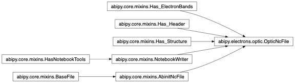
classmethod from_file(filepath)

Initialize the object from a netcdf file.

wmesh()

Frequency mesh in eV. Note that the same frequency-mesh is used for the different optical properties.

to_string(verbose=0)

String representation.

ebands()

abipy.electrons.ebands.ElectronBands object.

property structure

abipy.core.structure.Structure object.

has_linopt()

True if the ncfile contains Second Harmonic Generation tensor.

has_shg()

True if the ncfile contains Second Harmonic Generation tensor.

has_leo()

True if the ncfile contains the Linear Electro-optic tensor

close()

Close the file.

params()

OrderedDict with parameters that might be subject to convergence studies.

static get_linopt_latex_label(what, comp)

Return latex label for linear-optic quantities. Used in plots.

get_chi2_latex_label(key, what, comp)

Build latex label for chi2-related quantities. Used in plots.

plot_linear_epsilon(components='all', what='im', itemp=0, ax=None, xlims=None, with_xlabel=True, label=None, fontsize=12, **kwargs)

Plot components of the linear dielectric function.

Parameters

• components – List of cartesian tensor components to plot e.g. [“xx”, “xy”]. “all” if all components available on file should be plotted on the same ax.

• what – quantity to plot. “re” for real part, “im” for imaginary. Accepts also “abs”, “angle”.

• itemp – Temperature index.

• ax – matplotlib.axes.Axes or None if a new figure should be created.

• xlims – Set the data limits for the x-axis. Accept tuple e.g. (left, right) or scalar e.g. left. If left (right) is None, default values are used.

• with_xlabel – True if x-label should be added.

• label – True to add legend label to each curve.

• fontsize – Legend and label fontsize.

Returns: matplotlib.figure.Figure

Keyword arguments controlling the display of the figure:

kwargs	Meaning
title	Title of the plot (Default: None).
show	True to show the figure (default: True).
savefig	“abc.png” or “abc.eps” to save the figure to a file.
size_kwargs	Dictionary with options passed to fig.set_size_inches e.g. size_kwargs=dict(w=3, h=4)
tight_layout	True to call fig.tight_layout (default: False)
ax_grid	True (False) to add (remove) grid from all axes in fig. Default: None i.e. fig is left unchanged.
ax_annotate	Add labels to subplots e.g. (a), (b). Default: False
fig_close	Close figure. Default: False.

plot_linopt(select='all', itemp=0, xlims=None, **kwargs)

Subplots with all linear optic quantities selected by select at temperature itemp.

Parameters

• select –

• itemp – Temperature index.

• xlims – Set the data limits for the x-axis. Accept tuple e.g. (left, right) or scalar e.g. left. If left (right) is None, default values are used.

Returns: matplotlib.figure.Figure

Keyword arguments controlling the display of the figure:

kwargs	Meaning
title	Title of the plot (Default: None).
show	True to show the figure (default: True).
savefig	“abc.png” or “abc.eps” to save the figure to a file.
size_kwargs	Dictionary with options passed to fig.set_size_inches e.g. size_kwargs=dict(w=3, h=4)
tight_layout	True to call fig.tight_layout (default: False)
ax_grid	True (False) to add (remove) grid from all axes in fig. Default: None i.e. fig is left unchanged.
ax_annotate	Add labels to subplots e.g. (a), (b). Default: False
fig_close	Close figure. Default: False.

plot_chi2(key, components='all', what='abs', itemp=0, decompose=False, ax=None, xlims=None, with_xlabel=True, label=None, fontsize=12, **kwargs)

Low-level function to plot chi2 tensor.

Parameters

• key –

• components – List of cartesian tensor components to plot e.g. [“xxx”, “xyz”]. “all” if all components available on file should be plotted on the same ax.

• what – quantity to plot. “re” for real part, “im” for imaginary, Accepts also “abs”, “angle”.

• itemp – Temperature index.

• decompose – True to plot individual contributions.

• ax – matplotlib.axes.Axes or None if a new figure should be created.

• xlims – Set the data limits for the x-axis. Accept tuple e.g. (left, right) or scalar e.g. left. If left (right) is None, default values are used.

• with_xlabel – True to add x-label.

• label – True to add legend label to each curve.

• fontsize – Legend and label fontsize.

Returns: matplotlib.figure.Figure

Keyword arguments controlling the display of the figure:

kwargs	Meaning
title	Title of the plot (Default: None).
show	True to show the figure (default: True).
savefig	“abc.png” or “abc.eps” to save the figure to a file.
size_kwargs	Dictionary with options passed to fig.set_size_inches e.g. size_kwargs=dict(w=3, h=4)
tight_layout	True to call fig.tight_layout (default: False)
ax_grid	True (False) to add (remove) grid from all axes in fig. Default: None i.e. fig is left unchanged.
ax_annotate	Add labels to subplots e.g. (a), (b). Default: False
fig_close	Close figure. Default: False.

plot_shg(**kwargs)

Plot Second Harmonic Generation. See plot_chi2 for args supported.

Keyword arguments controlling the display of the figure:

kwargs	Meaning
title	Title of the plot (Default: None).
show	True to show the figure (default: True).
savefig	“abc.png” or “abc.eps” to save the figure to a file.
size_kwargs	Dictionary with options passed to fig.set_size_inches e.g. size_kwargs=dict(w=3, h=4)
tight_layout	True to call fig.tight_layout (default: False)
ax_grid	True (False) to add (remove) grid from all axes in fig. Default: None i.e. fig is left unchanged.
ax_annotate	Add labels to subplots e.g. (a), (b). Default: False
fig_close	Close figure. Default: False.

plot_leo(**kwargs)

Plot Linear Electro-optic. See plot_chi2 for args supported.

Keyword arguments controlling the display of the figure:

kwargs	Meaning
title	Title of the plot (Default: None).
show	True to show the figure (default: True).
savefig	“abc.png” or “abc.eps” to save the figure to a file.
size_kwargs	Dictionary with options passed to fig.set_size_inches e.g. size_kwargs=dict(w=3, h=4)
tight_layout	True to call fig.tight_layout (default: False)
ax_grid	True (False) to add (remove) grid from all axes in fig. Default: None i.e. fig is left unchanged.
ax_annotate	Add labels to subplots e.g. (a), (b). Default: False
fig_close	Close figure. Default: False.

yield_figs(**kwargs)

This function generates a predefined list of matplotlib figures with minimal input from the user. Used in abiview.py to get a quick look at the results.

write_notebook(nbpath=None)

Write a jupyter notebook to nbpath. If nbpath is None, a temporay file in the current working directory is created. Return path to the notebook.

class abipy.electrons.optic.OpticReader(filepath)

Bases: abipy.electrons.ebands.ElectronsReader

This object reads the results stored in the optic.nc file It provides helper function to access the most important quantities.

Inheritance Diagram

read_lineps(components, itemp=0)

Parameters

• components – List of cartesian tensor components to plot e.g. [“xx”, “xy”]. “all” if all components available on file should be plotted on the same ax.

• itemp – Temperature index.

read_tensor3_terms(key, components, itemp=0)

Parameters

• key – Name of the netcdf variable to read.

• components – List of cartesian tensor components to plot e.g. [“xxx”, “xyz”]. “all” if all components available on file should be plotted on the same ax.

• itemp – Temperature index.

Returns

OrderedDict mapping cartesian components e.g. “xyz” to data dictionary. Individual entries are listed in ALL_CHIS[key][“terms”]

class abipy.electrons.optic.OpticRobot(*args)

Bases: abipy.abio.robots.Robot, abipy.electrons.ebands.RobotWithEbands

This robot analyzes the results contained in multiple optic.nc files.

Inheritance Diagram

EXT = 'OPTIC'

computed_components_intersection()

Dictionary with the list of cartesian tensor components available in each file. Use keys from ALL_CHIS.

plot_linopt_convergence(components='all', what_list=('re', 'im'), sortby='nkpt', itemp=0, xlims=None, **kwargs)

Plot the convergence of the dielectric function tensor with respect to parameter defined by sortby.

Parameters

• components – List of cartesian tensor components to plot e.g. [“xx”, “xy”]. “all” if all components available on file should be plotted on the same ax.

• what_list – List of quantities to plot. “re” for real part, “im” for imaginary. Accepts also “abs”, “angle”.

• sortby – Define the convergence parameter, sort files and produce plot labels. Can be None, string or function. If None, no sorting is performed. If string, it’s assumed that the ncfile has an attribute with the same name and getattr is invoked. If callable, the output of callable(ncfile) is used.

• itemp – Temperature index.

• xlims – Set the data limits for the x-axis. Accept tuple e.g. (left, right) or scalar e.g. left. If left (right) is None, default values are used.

Returns: matplotlib.figure.Figure

Keyword arguments controlling the display of the figure:

kwargs	Meaning
title	Title of the plot (Default: None).
show	True to show the figure (default: True).
savefig	“abc.png” or “abc.eps” to save the figure to a file.
size_kwargs	Dictionary with options passed to fig.set_size_inches e.g. size_kwargs=dict(w=3, h=4)
tight_layout	True to call fig.tight_layout (default: False)
ax_grid	True (False) to add (remove) grid from all axes in fig. Default: None i.e. fig is left unchanged.
ax_annotate	Add labels to subplots e.g. (a), (b). Default: False
fig_close	Close figure. Default: False.

plot_shg_convergence(**kwargs)

Plot Second Harmonic Generation. See plot_convergence_rank3 for args supported.

Keyword arguments controlling the display of the figure:

kwargs	Meaning
title	Title of the plot (Default: None).
show	True to show the figure (default: True).
savefig	“abc.png” or “abc.eps” to save the figure to a file.
size_kwargs	Dictionary with options passed to fig.set_size_inches e.g. size_kwargs=dict(w=3, h=4)
tight_layout	True to call fig.tight_layout (default: False)
ax_grid	True (False) to add (remove) grid from all axes in fig. Default: None i.e. fig is left unchanged.
ax_annotate	Add labels to subplots e.g. (a), (b). Default: False
fig_close	Close figure. Default: False.

plot_leo_convergence(**kwargs)

Plot Linear electron-optic. See plot_convergence_rank3 for args supported.

Keyword arguments controlling the display of the figure:

kwargs	Meaning
title	Title of the plot (Default: None).
show	True to show the figure (default: True).
savefig	“abc.png” or “abc.eps” to save the figure to a file.
size_kwargs	Dictionary with options passed to fig.set_size_inches e.g. size_kwargs=dict(w=3, h=4)
tight_layout	True to call fig.tight_layout (default: False)
ax_grid	True (False) to add (remove) grid from all axes in fig. Default: None i.e. fig is left unchanged.
ax_annotate	Add labels to subplots e.g. (a), (b). Default: False
fig_close	Close figure. Default: False.

plot_convergence_rank3(key, components='all', itemp=0, what_list=('abs'), sortby='nkpt', decompose=False, xlims=None, **kwargs)

Plot convergence of arbitrary rank3 tensor. This is a low-level routine used in other plot methods.

Parameters

• key – Name of the quantity to analyze.

• components – List of cartesian tensor components to plot e.g. [“xxx”, “xyz”]. “all” if all components available on file should be plotted on the same ax.

• itemp – Temperature index.

• what_list – List of quantities to plot. “re” for real part, “im” for imaginary. Accepts also “abs”, “angle”.

• sortby – Define the convergence parameter, sort files and produce plot labels. Can be None, string or function. If None, no sorting is performed. If string, it’s assumed that the ncfile has an attribute with the same name and getattr is invoked. If callable, the output of callable(ncfile) is used.

• decompose – True to plot individual contributions.

• xlims – Set the data limits for the x-axis. Accept tuple e.g. (left, right) or scalar e.g. left. If left (right) is None, default values are used.

Returns: matplotlib.figure.Figure

Keyword arguments controlling the display of the figure:

kwargs	Meaning
title	Title of the plot (Default: None).
show	True to show the figure (default: True).
savefig	“abc.png” or “abc.eps” to save the figure to a file.
size_kwargs	Dictionary with options passed to fig.set_size_inches e.g. size_kwargs=dict(w=3, h=4)
tight_layout	True to call fig.tight_layout (default: False)
ax_grid	True (False) to add (remove) grid from all axes in fig. Default: None i.e. fig is left unchanged.
ax_annotate	Add labels to subplots e.g. (a), (b). Default: False
fig_close	Close figure. Default: False.

yield_figs(**kwargs)

This function generates a predefined list of matplotlib figures with minimal input from the user. Used in abiview.py to get a quick look at the results.

write_notebook(nbpath=None)

Write a jupyter notebook to nbpath. If nbpath is None, a temporay file in the current working directory is created. Return path to the notebook.

psps Module

PSPS file with tabulated data.

abipy.electrons.psps.mklabel(fsym, der, arg)

mklabel(f, 2, x) –> $f’’(x)$

abipy.electrons.psps.rescale(arr, scale=1.0)

abipy.electrons.psps.dataframe_from_pseudos(pseudos, index=None)

Build pandas dataframe with the most important info associated to a list of pseudos or a list of objects that can be converted into pseudos.

Parameters

• pseudos – List of objects that can be converted to pseudos.

• index – Index of the dataframe.

Return: pandas Dataframe.

class abipy.electrons.psps.PspsFile(filepath)

Bases: abipy.core.mixins.AbinitNcFile

Netcdf file with the tables used in Abinit to apply the pseudopotential part of the KS Hamiltonian.

Usage example:

with PspsFile("foo_PSPS.nc") as psps:
    psps.plot_tcore_rspace()

linestyles_der = ['-', '--', '-.', ':', ':', ':']

color_der = ['black', 'red', 'green', 'orange', 'cyan']

classmethod from_file(filepath)

Initialize the object from a Netcdf file

close()

Close the file.

params()

OrderedDict with parameters that might be subject to convergence studies.

plot(**kwargs)

Driver routine to plot several quantities on the same graph.

Parameters

ecut_ffnl – Max cutoff energy for ffnl plot (optional)

Return: matplotlib.figure.Figure

Keyword arguments controlling the display of the figure:

kwargs	Meaning
title	Title of the plot (Default: None).
show	True to show the figure (default: True).
savefig	“abc.png” or “abc.eps” to save the figure to a file.
size_kwargs	Dictionary with options passed to fig.set_size_inches e.g. size_kwargs=dict(w=3, h=4)
tight_layout	True to call fig.tight_layout (default: False)
ax_grid	True (False) to add (remove) grid from all axes in fig. Default: None i.e. fig is left unchanged.
ax_annotate	Add labels to subplots e.g. (a), (b). Default: False
fig_close	Close figure. Default: False.

plot_tcore_rspace(ax=None, ders=(0, 1, 2, 3), rmax=3.0, **kwargs)

Plot the model core and its derivatives in real space.

Parameters

• ax – matplotlib.axes.Axes or None if a new figure should be created.

• ders – Tuple used to select the derivatives to be plotted.

• rmax – Max radius for plot in Bohr. None is full grid is wanted.

Returns: matplotlib.figure.Figure

Keyword arguments controlling the display of the figure:

kwargs	Meaning
title	Title of the plot (Default: None).
show	True to show the figure (default: True).
savefig	“abc.png” or “abc.eps” to save the figure to a file.
size_kwargs	Dictionary with options passed to fig.set_size_inches e.g. size_kwargs=dict(w=3, h=4)
tight_layout	True to call fig.tight_layout (default: False)
ax_grid	True (False) to add (remove) grid from all axes in fig. Default: None i.e. fig is left unchanged.
ax_annotate	Add labels to subplots e.g. (a), (b). Default: False
fig_close	Close figure. Default: False.

plot_tcore_qspace(ax=None, ders=(0), with_fact=True, with_qn=0, **kwargs)

Plot the model core in q space

Parameters

• ax – matplotlib.axes.Axes or None if a new figure should be created.

• ders – Tuple used to select the derivatives to be plotted.

• with_qn –

Returns: matplotlib.figure.Figure

Keyword arguments controlling the display of the figure:

kwargs	Meaning
title	Title of the plot (Default: None).
show	True to show the figure (default: True).
savefig	“abc.png” or “abc.eps” to save the figure to a file.
size_kwargs	Dictionary with options passed to fig.set_size_inches e.g. size_kwargs=dict(w=3, h=4)
tight_layout	True to call fig.tight_layout (default: False)
ax_grid	True (False) to add (remove) grid from all axes in fig. Default: None i.e. fig is left unchanged.
ax_annotate	Add labels to subplots e.g. (a), (b). Default: False
fig_close	Close figure. Default: False.

plot_vlocq(ax=None, ders=(0), with_qn=0, with_fact=True, **kwargs)

Plot the local part of the pseudopotential in q space.

Parameters

• ax – matplotlib.axes.Axes or None if a new figure should be created.

• ders – Tuple used to select the derivatives to be plotted.

• with_qn –

Returns: matplotlib.figure.Figure

Keyword arguments controlling the display of the figure:

kwargs	Meaning
title	Title of the plot (Default: None).
show	True to show the figure (default: True).
savefig	“abc.png” or “abc.eps” to save the figure to a file.
size_kwargs	Dictionary with options passed to fig.set_size_inches e.g. size_kwargs=dict(w=3, h=4)
tight_layout	True to call fig.tight_layout (default: False)
ax_grid	True (False) to add (remove) grid from all axes in fig. Default: None i.e. fig is left unchanged.
ax_annotate	Add labels to subplots e.g. (a), (b). Default: False
fig_close	Close figure. Default: False.

plot_ffspl(ax=None, ecut_ffnl=None, ders=(0), with_qn=0, with_fact=False, **kwargs)

Plot the nonlocal part of the pseudopotential in q-space.

Parameters

• ax – matplotlib.axes.Axes or None if a new figure should be created.

• ecut_ffnl – Max cutoff energy for ffnl plot (optional)

• ders – Tuple used to select the derivatives to be plotted.

• with_qn –

Returns: matplotlib.figure.Figure

Keyword arguments controlling the display of the figure:

kwargs	Meaning
title	Title of the plot (Default: None).
show	True to show the figure (default: True).
savefig	“abc.png” or “abc.eps” to save the figure to a file.
size_kwargs	Dictionary with options passed to fig.set_size_inches e.g. size_kwargs=dict(w=3, h=4)
tight_layout	True to call fig.tight_layout (default: False)
ax_grid	True (False) to add (remove) grid from all axes in fig. Default: None i.e. fig is left unchanged.
ax_annotate	Add labels to subplots e.g. (a), (b). Default: False
fig_close	Close figure. Default: False.

compare(others, **kwargs)

Produce matplotlib plot comparing self with another list of pseudos others.

Keyword arguments controlling the display of the figure:

kwargs	Meaning
title	Title of the plot (Default: None).
show	True to show the figure (default: True).
savefig	“abc.png” or “abc.eps” to save the figure to a file.
size_kwargs	Dictionary with options passed to fig.set_size_inches e.g. size_kwargs=dict(w=3, h=4)
tight_layout	True to call fig.tight_layout (default: False)
ax_grid	True (False) to add (remove) grid from all axes in fig. Default: None i.e. fig is left unchanged.
ax_annotate	Add labels to subplots e.g. (a), (b). Default: False
fig_close	Close figure. Default: False.

class abipy.electrons.psps.PspsReader(filepath)

Bases: abipy.iotools.ETSF_Reader

This object reads the results stored in the PSPS file produced by ABINIT. It provides helper function to access the most important quantities.

read_coresd(rmax=None)

Read the core charges and derivatives for the different types of atoms.

Parameters

rmax – Maximum radius in Bohr. If None, data on the full grid is returned.

Returns

List of ntypat arrays. Each array contains the linear meshes in real space. coresd: List with nytpat arrays of shape [6, npts].

(np.zeros. np.zeros) if core charge is not present

Return type

meshes

xccc1d[ntypat6,n1xccc*(1-usepaw)]

Norm-conserving psps only The component xccc1d(n1xccc,1,ntypat) is the pseudo-core charge for each type of atom, on the radial grid. The components xccc1d(n1xccc,ideriv,ntypat) give the ideriv-th derivative of the pseudo-core charge with respect to the radial distance.

read_tcorespl()

Returns

Linear q-mesh in G-space tcorespl:

Return type

qmesh

tcorespl[ntypat, 2, mqgrid_vl] Gives the pseudo core density in reciprocal space on a regular grid. Only if has_tcore

read_vlspl()

Returns

Linear q-mesh in G-space vlspl:

Return type

qmesh

vlspl[2, ntypat, mqgrid_vl] Gives, on the radial grid, the local part of each type of psp.

read_projectors()

ffspl(ntypat, lnmax, 2, mqgrid_ff] Gives, on the radial grid, the different non-local projectors, in both the norm-conserving case, and the PAW case

get_lnlist_for_type(itypat)

Return a list of (l, n) indices for this atom type.

class abipy.electrons.psps.VnlProjector(itypat, ln, ekb, qmesh, data)

Bases: object

Data and parameters associated to a non-local projector.

property values

Values of the projector in q-space.

property der2

Second order derivative.

property ecuts

List of cutoff energies corresponding to self.qmesh.

property sign_sqrtekb

scissors Module

Scissors operator.

class abipy.electrons.scissors.Scissors(func_list, domains, residues, bounds=None)

Bases: object

This object represents an energy-dependent scissors operator. The operator is defined by a list of domains (energy intervals) and a list of functions defined in these domains. The domains should fulfill the constraints documented in the main constructor.

Note

eV units are assumed.

The standard way to create this object is via the methods provided by the factory class ScissorBuilder. Once the instance has been created, one can correct the band structure by calling the apply method.

Error

alias of abipy.electrons.scissors.ScissorsError

apply(eig)

Correct the eigenvalue eig (eV units).

class abipy.electrons.scissors.ScissorsBuilder(qps_spin, sigres_ebands)

Bases: object

This object facilitates the creation of Scissors instances.

Usage:

builder = ScissorsBuilder.from_file(“out_SIGRES.nc”)

# To plot the QP results as function of the KS energy: builder.plot_qpe_vs_e0()

# To select the domains esplicitly (optional but highly recommended) builder.build(domains_spin=[[-10, 6.02], [6.1, 20]])

# To compare the fitted results with the ab-initio data: builder.plot_fit()

# To plot the corrected bands: builder.plot_qpbands(abidata.ref_file(“si_nscf_WFK.nc”))

classmethod from_file(filepath)

Generate object from (SIGRES.nc) file. Main entry point for client code.

classmethod pickle_load(filepath)

Load the object from a pickle file.

pickle_dump(filepath, protocol=- 1)

Save the object in Pickle format

property nsppol

Number of spins.

property e0min

Minimum KS energy in eV (takes into account spin)

property e0max

Maximum KS energy in eV (takes into account spin)

property scissors_spin

Returns a tuple of Scissors indexed by the spin value.

build(domains_spin=None, bounds_spin=None, k=3)

Build the scissors operator.

Parameters

• domains_spin – list of domains in eV for each spin. If domains is None, domains are computed automatically from the sigres bands (two domains separated by the middle of the gap).

• bounds_spin – Options specifying the boundary conditions (not used at present)

• k – Parameter defining the order of the fit.

plot_qpe_vs_e0(with_fields='all', **kwargs)

Plot the quasiparticle corrections as function of the KS energy.

Keyword arguments controlling the display of the figure:

kwargs	Meaning
title	Title of the plot (Default: None).
show	True to show the figure (default: True).
savefig	“abc.png” or “abc.eps” to save the figure to a file.
size_kwargs	Dictionary with options passed to fig.set_size_inches e.g. size_kwargs=dict(w=3, h=4)
tight_layout	True to call fig.tight_layout (default: False)
ax_grid	True (False) to add (remove) grid from all axes in fig. Default: None i.e. fig is left unchanged.
ax_annotate	Add labels to subplots e.g. (a), (b). Default: False
fig_close	Close figure. Default: False.

plot_fit(ax=None, fontsize=8, **kwargs)

Compare fit functions with input quasi-particle corrections.

Parameters

• ax – matplotlib.axes.Axes or None if a new figure should be created.

• fontsize – fontsize for titles and legend.

Return: matplotlib.figure.Figure

Keyword arguments controlling the display of the figure:

kwargs	Meaning
title	Title of the plot (Default: None).
show	True to show the figure (default: True).
savefig	“abc.png” or “abc.eps” to save the figure to a file.
size_kwargs	Dictionary with options passed to fig.set_size_inches e.g. size_kwargs=dict(w=3, h=4)
tight_layout	True to call fig.tight_layout (default: False)
ax_grid	True (False) to add (remove) grid from all axes in fig. Default: None i.e. fig is left unchanged.
ax_annotate	Add labels to subplots e.g. (a), (b). Default: False
fig_close	Close figure. Default: False.

plot_qpbands(bands_filepath, bands_label=None, dos_filepath=None, dos_args=None, **kwargs)

Correct the energies found in the netcdf file bands_filepath and plot the band energies (both the initial and the corrected ones) with matplotlib. The plot contains the KS and the QP DOS if dos_filepath is not None.

Parameters

• bands_filepath – Path to the netcdf file containing the initial KS energies to be corrected.

• String used to label the KS bands in the plot. (bands_label) –

• dos_filepath – Optional path to a netcdf file with the initial KS energies on a homogeneous k-mesh (used to compute the KS and the QP dos)

• dos_args – Dictionary with the arguments passed to get_dos to compute the DOS Used if dos_filepath is not None.

• kwargs – Options passed to the plotter.

Return: matplotlib.figure.Figure

scr Module

Objects to analyze the screening files produced by the GW code (optdriver 3).

class abipy.electrons.scr.ScrFile(filepath)

Bases: abipy.core.mixins.AbinitNcFile, abipy.core.mixins.Has_Header, abipy.core.mixins.Has_Structure, abipy.core.mixins.NotebookWriter

This object provides an interface to the SCR.nc file produced by the GW code.

Usage example:

with ScrFile("foo_SCR.nc") as ncfile:
    print(ncfile)
    ncfile.plot_emacro()

Inheritance Diagram

classmethod from_file(filepath)

Initialize the object from a Netcdf file

close()

Close the file.

to_string(verbose=0)

String representation.

property structure

abipy.core.structure.Structure object.

property kpoints

List of k-points in the dielectric function.

ebands()

abipy.electrons.ebands.ElectronBands object with the single-particle energies used to compute the screening.

property ng

Number of G-vectors in screening matrices.

property wpoints

Array of complex numbers with the frequencies of the dielectric function in Hartree.

property nw

Total number of frequencies.

property nrew

Number of real frequencies.

property nimw

Number of imaginary frequencies.

property netcdf_name

The netcdf name associated to the data on disk.

params()

monty.collections.AttrDict with the most important parameters used to compute the screening keys can be accessed with the dot notation i.e. params.zcut.

plot_emacro(cplx_mode='re-im', ax=None, xlims=None, fontsize=12, **kwargs)

Plot the macroscopic dielectric function with local-field effects.

Parameters

• cplx_mode – string defining the data to print. Possible choices are (case-insensitive): “re” for the real part. “im” for the imaginary part. “abs” for the absolute value. “angle” will display the phase of the complex number in radians. Options can be concatenated with - e.g. re-im.

• xlims – Set the data limits for the x-axis in eV. Accept tuple e.g. (left, right) or scalar e.g. left. If left (right) is None, default values are used.

• ax – matplotlib.axes.Axes or None if a new figure should be created.

• fontsize – Legend and title fontsize.

Returns

matplotlib.figure.Figure

Keyword arguments controlling the display of the figure:

kwargs	Meaning
title	Title of the plot (Default: None).
show	True to show the figure (default: True).
savefig	“abc.png” or “abc.eps” to save the figure to a file.
size_kwargs	Dictionary with options passed to fig.set_size_inches e.g. size_kwargs=dict(w=3, h=4)
tight_layout	True to call fig.tight_layout (default: False)
ax_grid	True (False) to add (remove) grid from all axes in fig. Default: None i.e. fig is left unchanged.
ax_annotate	Add labels to subplots e.g. (a), (b). Default: False
fig_close	Close figure. Default: False.

plot_eelf(ax=None, xlims=None, fontsize=12, **kwargs)

Plot electron energy loss function.

Parameters

• ax – matplotlib.axes.Axes or None if a new figure should be created.

• xlims – Set the data limits for the x-axis in eV. Accept tuple e.g. (left, right) or scalar e.g. left. If left (right) is None, default values are used

• fontsize – Legend and label fontsize:

Returns: matplotlib.figure.Figure

Keyword arguments controlling the display of the figure:

kwargs	Meaning
title	Title of the plot (Default: None).
show	True to show the figure (default: True).
savefig	“abc.png” or “abc.eps” to save the figure to a file.
size_kwargs	Dictionary with options passed to fig.set_size_inches e.g. size_kwargs=dict(w=3, h=4)
tight_layout	True to call fig.tight_layout (default: False)
ax_grid	True (False) to add (remove) grid from all axes in fig. Default: None i.e. fig is left unchanged.
ax_annotate	Add labels to subplots e.g. (a), (b). Default: False
fig_close	Close figure. Default: False.

yield_figs(**kwargs)

This function generates a predefined list of matplotlib figures with minimal input from the user. Used in abiview.py to get a quick look at the results.

write_notebook(nbpath=None)

Write a jupyter notebook to nbpath. If nbpath is None, a temporay file in the current working directory is created. Return path to the notebook.

class abipy.electrons.scr.ScrReader(filepath)

Bases: abipy.iotools.ETSF_Reader

This object reads the results stored in the SCR (Screening) file produced by ABINIT. It provides helper functions to access the most important quantities.

double inverse_dielectric_function(number_of_qpoints_dielectric_function, number_of_frequencies_dielectric_function, number_of_spins, number_of_spins, number_of_coefficients_dielectric_function, number_of_coefficients_dielectric_function, complex)

Inheritance Diagram

read_params()

Read the most important parameters used to compute the screening i.e. the parameters that may be subject to convergence studies.

Returns

monty.collections.AttrDict a dictionary whose keys can be accessed with the dot notation i.e. d.key.

read_emacro_lf(kpoint=(0, 0, 0))

Read the macroscopic dielectric function with local field effects 1 / em1_{0,0)(kpoint, omega).

Return: abipy.core.func1d.Function1D object.

read_emacro_nlf(kpoint=(0, 0, 0))

Read the macroscopic dielectric function without local field effects e_{0,0)(kpoint, omega).

Return: abipy.core.func1d.Function1D

Warning

This function performs the inversion of e-1 to get e. that can be quite expensive and memory demanding for large matrices!

read_eelf(kpoint=(0, 0, 0))

Read electron energy loss function

• Im(1/ emacro)

Return: abipy.core.func1d.Function1D object.

read_wggmat(kpoint, spin1=0, spin2=0, cls=None)

Read data at the given k-point and return an instance of cls where cls is a subclass of _AwggMatrix

find_kpoint_fileindex(kpoint)

Returns the k-point and the index of the k-point in the netcdf file. Accepts abipy.core.kpoints.Kpoint instance or integer.

read_wslice(kpoint, ig1=0, ig2=0, spin1=0, spin2=0)

Read slice along the frequency dimension.

class abipy.electrons.scr.Polarizability(wpoints, gsphere, wggmat, inord='C')

Bases: abipy.electrons.scr._AwggMatrix

Inheritance Diagram

netcdf_name = 'polarizability'

latex_name = '\\tilde chi'

class abipy.electrons.scr.DielectricFunction(wpoints, gsphere, wggmat, inord='C')

Bases: abipy.electrons.scr._AwggMatrix

Inheritance Diagram

netcdf_name = 'dielectric_function'

latex_name = '\\epsilon'

class abipy.electrons.scr.InverseDielectricFunction(wpoints, gsphere, wggmat, inord='C')

Bases: abipy.electrons.scr._AwggMatrix

Inheritance Diagram

netcdf_name = 'inverse_dielectric_function'

latex_name = '\\epsilon^{-1}'