waves Package

Contents

• waves Package

  • waves Package

  • pwwave Module

  • wfkfile Module

waves Package

pwwave Module

This module contains the class describing a planewave wavefunction.

class abipy.waves.pwwave.PWWaveFunction(structure, nspinor, spin, band, gsphere, ug)

Bases: abipy.waves.pwwave.WaveFunction

This object describes a wavefunction expressed in a plane-wave basis set.

Inheritance Diagram

norm2(space='g')

Return \(||\psi||^2\) computed in G- or r-space.

space: Integration space. Possible values [“g”, “gsphere”, “r”]

if “g” or “r” the scalar product is computed in G- or R-space on the FFT box. if “gsphere” the integration is done on the G-sphere.

braket(other, space='g')

Returns the scalar product <u1|u2> of the periodic part of two wavefunctions computed in G-space or r-space, depending on the value of space. Note that selection rules introduced by k-points is not taken into accout.

Parameters

• other – Other wave (right-hand side)

• space – Integration space. Possible values [“g”, “gsphere”, “r”] if “g” or “r” the scalar product is computed in G- or R-space on the FFT box. if “gsphere” the integration is done on the G-sphere. Note that this option assumes that self and other have the same list of G-vectors.

get_interpolator()

Return an interpolator object that interpolates periodic functions in real space.

plot_line(point1, point2, num=200, with_krphase=False, cartesian=False, ax=None, fontsize=12, **kwargs)

Plot (interpolated) wavefunction in real space along a line defined by point1 and point2.

Parameters

• point1 – First point of the line. Accepts 3d vector or integer. The vector is in reduced coordinates unless cartesian is True. If integer, the first point of the line is given by the i-th site of the structure e.g. point1=0, point2=1 gives the line passing through the first two atoms.

• point2 – Second point of the line. Same API as point1.

• num – Number of points sampled along the line.

• with_krphase – True to include the \(e^{ikr}\) phase-factor.

• cartesian – By default, point1 and point1 are interpreted as points in fractional coordinates (if not integers). Use True to pass points in cartesian coordinates.

• ax – matplotlib.axes.Axes or None if a new figure should be created.

• fontsize – legend and title fontsize.

Return: matplotlib.figure.Figure

Keyword arguments controlling the display of the figure:

kwargs	Meaning
title	Title of the plot (Default: None).
show	True to show the figure (default: True).
savefig	“abc.png” or “abc.eps” to save the figure to a file.
size_kwargs	Dictionary with options passed to fig.set_size_inches e.g. size_kwargs=dict(w=3, h=4)
tight_layout	True to call fig.tight_layout (default: False)
ax_grid	True (False) to add (remove) grid from all axes in fig. Default: None i.e. fig is left unchanged.
ax_annotate	Add labels to subplots e.g. (a), (b). Default: False
fig_close	Close figure. Default: False.

plot_line_neighbors(site_index, radius, num=200, with_krphase=False, max_nn=10, fontsize=12, **kwargs)

Plot (interpolated) density/potential in real space along the lines connecting an atom specified by site_index and all neighbors within a sphere of given radius.

Parameters

• site_index – Index of the atom in the structure.

• radius – Radius of the sphere in Angstrom.

• num – Number of points sampled along the line.

• with_krphase – True to include the \(e^{ikr}\) phase-factor.

• max_nn – By default, only the first max_nn neighbors are showed.

• fontsize – legend and label fontsize.

Return: matplotlib.figure.Figure

Keyword arguments controlling the display of the figure:

kwargs	Meaning
title	Title of the plot (Default: None).
show	True to show the figure (default: True).
savefig	“abc.png” or “abc.eps” to save the figure to a file.
size_kwargs	Dictionary with options passed to fig.set_size_inches e.g. size_kwargs=dict(w=3, h=4)
tight_layout	True to call fig.tight_layout (default: False)
ax_grid	True (False) to add (remove) grid from all axes in fig. Default: None i.e. fig is left unchanged.
ax_annotate	Add labels to subplots e.g. (a), (b). Default: False
fig_close	Close figure. Default: False.

export_ur2(filename, visu=None)

Export \(|u(r)|^2\) to file filename.

Parameters

• filename – String specifying the file path and the file format. The format is defined by the file extension. filename=”prefix.xsf”, for example, will produce a file in XSF format. An empty prefix, e.g. “.xsf” makes the code use a temporary file.

• visu – Visualizer subclass. By default, this method returns the first available visualizer that supports the given file format. If visu is not None, an instance of visu is returned. See Visualizer for the list of applications and formats supported.

Returns

Instance of Visualizer

visualize_ur2(appname='vesta')

Visualize \(|u(r)|^2|\).

See Visualizer for the list of applications and formats supported.

wfkfile Module

Wavefunction file.

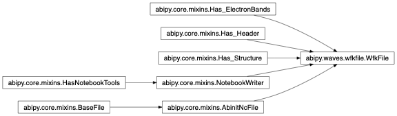
class abipy.waves.wfkfile.WfkFile(filepath)

Bases: abipy.core.mixins.AbinitNcFile, abipy.core.mixins.Has_Header, abipy.core.mixins.Has_Structure, abipy.core.mixins.Has_ElectronBands, abipy.core.mixins.NotebookWriter

This object provides a simplified interface to access and analyze the data stored in the WFK.nc file produced by ABINIT.

Usage example:

wfk = WfkFile("foo_WFK.nc")

# Plot band energies.
wfk.ebands.plot_ebands()

# Visualize crystalline structure with vesta.
wfk.visualize_structure_with("vesta")

# Visualize u(r)**2 with vesta.
wfk.visualize_ur2(spin=0, kpoint=0, band=0, appname="vesta")

# Get a wavefunction.
wave = wfk.get_wave(spin=0, kpoint=[0, 0, 0], band=0)

Inheritance Diagram

close()

Close the file.

params()

OrderedDict with parameters that might be subject to convergence studies.

property structure

abipy.core.structure.Structure object.

property ebands

abipy.electrons.ebands.ElectronBands object

property nkpt

Number of k-points.

property gspheres

List of GSphere objects ordered by k-points.

to_string(verbose=0)

String representation

Parameters

verbose – verbosity level.

kindex(kpoint)

The index of the k-point in the file. Accepts Kpoint object or int.

get_wave(spin, kpoint, band)

Read and return the wavefunction with the given spin, band and kpoint.

Parameters

• spin – spin index. Must be in (0, 1)

• kpoint – Either Kpoint instance or integer giving the sequential index in the IBZ (C-convention).

• band – band index.

• returns – WaveFunction instance.

export_ur2(filepath, spin, kpoint, band, visu=None)

Export \(|u(r)|^2\) on file filename.

Returns

Instance of Visualizer

visualize_ur2(spin, kpoint, band, appname='vesta')

Visualize \(|u(r)|^2\) with visualizer. See Visualizer for the list of applications and formats supported.

ipw_visualize_widget()

Return an ipython widget with controllers to visualize the wavefunctions.

Warning

It seems there’s a bug with Vesta on MacOs if the user tries to open multiple wavefunctions as the tab in vesta is not updated!

yield_figs(**kwargs)

This function generates a predefined list of matplotlib figures with minimal input from the user. Used in abiview.py to get a quick look at the results.

write_notebook(nbpath=None)

Write an ipython notebook to nbpath. If nbpath is None, a temporay file in the current working directory is created. Return path to the notebook.