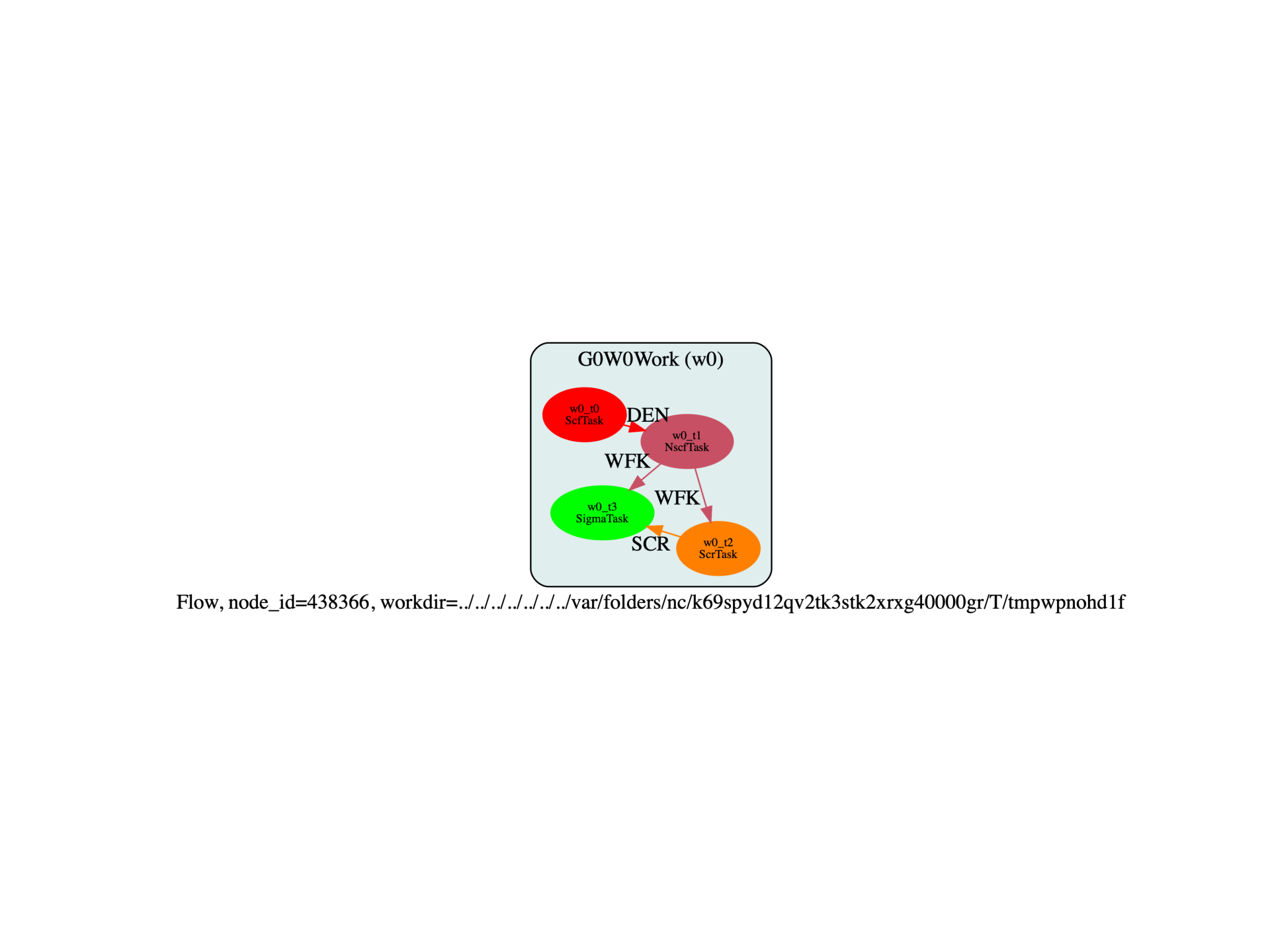
G0W0 Flow with factory functions

G0W0 corrections with the HT interface.

import sys
import os
import abipy.data as abidata
import abipy.flowtk as flowtk
from abipy import abilab


def build_flow(options):
    # Init structure and pseudos.
    structure = abilab.Structure.from_file(abidata.cif_file("si.cif"))
    pseudos = abidata.pseudos("14si.pspnc")

    # Working directory (default is the name of the script with '.py' removed and "run_" replaced by "flow_")
    if not options.workdir:
        options.workdir = os.path.basename(sys.argv[0]).replace(".py", "").replace("run_", "flow_")

    # Initialize the flow.
    flow = flowtk.Flow(options.workdir, manager=options.manager)

    scf_kppa = 120
    nscf_nband = 40
    ecut, ecuteps, ecutsigx = 6, 2, 4
    #scr_nband = 50
    #sigma_nband = 50

    multi = abilab.g0w0_with_ppmodel_inputs(
        structure, pseudos, scf_kppa, nscf_nband, ecuteps, ecutsigx,
        ecut=ecut, shifts=(0, 0, 0), # By default the k-mesh is shifted! TODO: Change default?
        accuracy="normal", spin_mode="unpolarized", smearing=None,
        #ppmodel="godby", charge=0.0, scf_algorithm=None, inclvkb=2, scr_nband=None,
        #sigma_nband=None, gw_qprange=1):
    )
    #multi.set_vars(paral_kgb=1)

    scf_input, nscf_input, scr_input, sigma_input = multi.split_datasets()
    work = flowtk.G0W0Work(scf_input, nscf_input, scr_input, sigma_input)
    flow.register_work(work)

    return flow


# This block generates the thumbnails in the Abipy gallery.
# You can safely REMOVE this part if you are using this script for production runs.
if os.getenv("READTHEDOCS", False):
    __name__ = None
    import tempfile
    options = flowtk.build_flow_main_parser().parse_args(["-w", tempfile.mkdtemp()])
    build_flow(options).graphviz_imshow()


@flowtk.flow_main
def main(options):
    """
    This is our main function that will be invoked by the script.
    flow_main is a decorator implementing the command line interface.
    Command line args are stored in `options`.
    """
    return build_flow(options)


if __name__ == "__main__":
    sys.exit(main())

Run the script with:

run_ht_si_g0w0ppm.py -s

The last task w0_t3 is the SigmaTask who has produced a netcdf file with the GW results as you can we with the command:

abirun.py flow_ht_si_g0w0ppm/ listext SIGRES

Let’s print the QP results with:

abiopen.py flow_ht_si_g0w0ppm/w0/t3/outdata/out_SIGRES.nc -p

================================= File Info =================================
Name: out_SIGRES.nc
Directory: /Users/gmatteo/git_repos/abipy/abipy/examples/flows/flow_ht_si_g0w0ppm/w0/t3/outdata
Size: 254.07 kb
Access Time: Sat Dec  9 19:16:05 2017
Modification Time: Sat Dec  9 15:16:15 2017
Change Time: Sat Dec  9 15:16:15 2017

================================= Structure =================================
Full Formula (Si2)
Reduced Formula: Si
abc   :   3.866975   3.866975   3.866975
angles:  60.000000  60.000000  60.000000
Sites (2)
  #  SP       a     b     c
---  ----  ----  ----  ----
  0  Si    0     0     0
  1  Si    0.25  0.25  0.25

Abinit Spacegroup: spgid: 0, num_spatial_symmetries: 48, has_timerev: True, symmorphic: True

============================== Kohn-Sham bands ==============================
Number of electrons: 8.0, Fermi level: 5.963 [eV]
nsppol: 1, nkpt: 8, mband: 40, nspinor: 1, nspden: 1
smearing scheme: none, tsmear_eV: 0.272, occopt: 1
Direct gap:
    Energy: 2.512 [eV]
    Initial state: spin=0, kpt=[+0.000, +0.000, +0.000], weight: 0.016, band=3, eig=5.640, occ=2.000
    Final state:   spin=0, kpt=[+0.000, +0.000, +0.000], weight: 0.016, band=4, eig=8.152, occ=0.000
Fundamental gap:
    Energy: 0.646 [eV]
    Initial state: spin=0, kpt=[+0.000, +0.000, +0.000], weight: 0.016, band=3, eig=5.640, occ=2.000
    Final state:   spin=0, kpt=[+0.500, +0.500, +0.000], weight: 0.047, band=4, eig=6.286, occ=0.000
Bandwidth: 11.867 [eV]
Valence minimum located at:
    spin=0, kpt=[+0.000, +0.000, +0.000], weight: 0.016, band=0, eig=-6.227, occ=2.000
Valence maximum located at:
    spin=0, kpt=[+0.000, +0.000, +0.000], weight: 0.016, band=3, eig=5.640, occ=2.000

============================ QP direct gaps in eV ============================
QP_dirgap: 3.000 for K-point: [+0.000, +0.000, +0.000], spin: 0
QP_dirgap: 3.087 for K-point: [+0.250, +0.000, +0.000], spin: 0
QP_dirgap: 3.068 for K-point: [+0.500, +0.000, +0.000], spin: 0
QP_dirgap: 3.421 for K-point: [+0.250, +0.250, +0.000], spin: 0
QP_dirgap: 4.165 for K-point: [+0.500, +0.250, +0.000], spin: 0
QP_dirgap: 4.206 for K-point: [-0.250, +0.250, +0.000], spin: 0
QP_dirgap: 4.003 for K-point: [+0.500, +0.500, +0.000], spin: 0
QP_dirgap: 8.683 for K-point: [-0.250, +0.500, +0.250], spin: 0

============== QP results for each k-point and spin (All in eV) ==============
K-point: [+0.000, +0.000, +0.000], spin: 0
   band     e0    qpe  qpe_diago   vxcme  sigxme  sigcmee0  vUme    ze0
1     1  5.640  5.547      5.520 -11.156 -12.870     1.594   0.0  0.776
2     2  5.640  5.547      5.521 -11.156 -12.870     1.594   0.0  0.776
3     3  5.640  5.547      5.521 -11.156 -12.870     1.594   0.0  0.776
4     4  8.152  8.547      8.662  -9.969  -5.622    -3.837   0.0  0.774
5     5  8.152  8.547      8.662  -9.969  -5.622    -3.837   0.0  0.774
6     6  8.152  8.547      8.662  -9.969  -5.622    -3.837   0.0  0.774

K-point: [+0.250, +0.000, +0.000], spin: 0
   band     e0    qpe  qpe_diago   vxcme  sigxme  sigcmee0  vUme    ze0
2     2  4.870  4.751      4.716 -10.936 -12.831     1.741   0.0  0.772
3     3  4.870  4.751      4.716 -10.936 -12.831     1.741   0.0  0.772
4     4  7.449  7.838      7.949 -10.031  -5.725    -3.806   0.0  0.778
5     5  9.108  9.534      9.660 -10.013  -5.381    -4.079   0.0  0.771
6     6  9.108  9.534      9.660 -10.013  -5.381    -4.079   0.0  0.771

K-point: [+0.500, +0.000, +0.000], spin: 0
   band     e0    qpe  qpe_diago   vxcme  sigxme  sigcmee0  vUme    ze0
2     2  4.431  4.282      4.238 -10.908 -13.077     1.976   0.0  0.769
3     3  4.431  4.282      4.238 -10.908 -13.077     1.976   0.0  0.769
4     4  6.972  7.350      7.456 -10.016  -5.844    -3.687   0.0  0.781
5     5  8.982  9.410      9.534  -9.621  -4.942    -4.127   0.0  0.775
6     6  8.982  9.410      9.534  -9.621  -4.942    -4.127   0.0  0.775

K-point: [+0.250, +0.250, +0.000], spin: 0
   band     e0    qpe  qpe_diago   vxcme  sigxme  sigcmee0  vUme    ze0
2     2  3.743  3.571      3.518 -10.603 -12.883     2.056   0.0  0.764
3     3  3.743  3.571      3.518 -10.603 -12.883     2.056   0.0  0.764
4     4  6.692  6.993      7.076  -9.352  -5.373    -3.595   0.0  0.783
5     5  8.669  9.035      9.139  -9.203  -4.548    -4.184   0.0  0.779

K-point: [+0.500, +0.250, +0.000], spin: 0
   band      e0     qpe  qpe_diago   vxcme  sigxme  sigcmee0  vUme    ze0
2     2   2.099   1.893      1.825 -10.130 -12.839     2.435   0.0  0.752
3     3   3.427   3.242      3.184 -10.596 -13.077     2.238   0.0  0.761
4     4   7.086   7.408      7.496  -9.224  -5.065    -3.748   0.0  0.784
5     5  10.015  10.397     10.510  -9.594  -4.730    -4.369   0.0  0.771

K-point: [-0.250, +0.250, +0.000], spin: 0
   band      e0     qpe  qpe_diago   vxcme  sigxme  sigcmee0  vUme    ze0
2     2   1.887   1.667      1.594  -9.982 -12.769     2.493   0.0  0.751
3     3   4.302   4.157      4.113 -10.820 -12.927     1.917   0.0  0.769
4     4   7.983   8.363      8.470  -9.567  -5.113    -3.966   0.0  0.779
5     5  10.350  10.800     10.942 -10.046  -4.859    -4.595   0.0  0.760

K-point: [+0.500, +0.500, +0.000], spin: 0
   band     e0    qpe  qpe_diago   vxcme  sigxme  sigcmee0  vUme    ze0
2     2  2.784  2.567      2.497 -10.480 -13.270     2.503   0.0  0.755
3     3  2.784  2.567      2.497 -10.480 -13.270     2.503   0.0  0.755
4     4  6.286  6.571      6.647  -9.003  -5.038    -3.603   0.0  0.787
5     5  6.286  6.571      6.647  -9.003  -5.038    -3.603   0.0  0.787

K-point: [-0.250, +0.500, +0.250], spin: 0
   band     e0     qpe  qpe_diago  vxcme  sigxme  sigcmee0  vUme    ze0
2     2  1.787   1.557      1.481 -9.917 -12.751     2.527   0.0  0.749
3     3  1.787   1.557      1.481 -9.917 -12.751     2.527   0.0  0.749
4     4  9.875  10.241     10.347 -9.523  -4.876    -4.176   0.0  0.775
5     5  9.875  10.241     10.347 -9.523  -4.876    -4.176   0.0  0.775

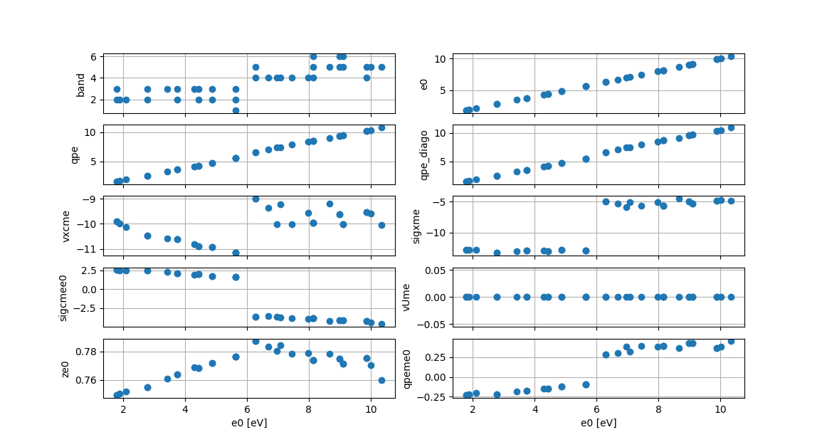
we can also plot the QP data as function of the initial KS energy with ipython:

abiopen.py flow_ht_si_g0w0ppm/w0/t3/outdata/out_SIGRES.nc

In [1]: %matplotlib
In [2]: abifile.plot_qps_vs_e0()