Relaxation with different k-meshes

In this example, we employ the relaxation algorithms implemented in Abinit (ionmov and optcell) to find the equilibrium configuration of GaN (atomic positions and lattice vectors). The relaxation is performed with different k-meshes to monitor the convergence of the results. You will observe a change of the equilibrium parameters with respect to the k-point mesh.

Note the we are using pseudopotentials generated with the GGA which tends to overestimate the lattice parameters and ecut is way too low. If you replace GGA with LDA, you will observe that LDA tends to underestimate the parameters.

import sys
import os

import abipy.abilab as abilab
import abipy.flowtk as flowtk
import abipy.data as abidata


def build_flow(options):
    """
    Build and return a flow performing structural relaxations with different k-point samplings.
    """
    # Set working directory (default is the name of the script with '.py' removed and "run_" replaced by "flow_")
    if not options.workdir:
        options.workdir = os.path.basename(sys.argv[0]).replace(".py", "").replace("run_", "flow_")

    # List of k-meshes.
    ngkpt_list = [
        [3, 3, 2],
        [6, 6, 4],
        [8, 8, 6],
    ]

    structure = abilab.Structure.from_file(abidata.cif_file("gan2.cif"))
    pseudos = abidata.pseudos("Ga.oncvpsp", "N.oncvpsp")

    # Build multidataset.
    multi = abilab.MultiDataset(structure=structure, pseudos=pseudos, ndtset=len(ngkpt_list))

    # Set global variables for structural relaxation. Note dilatmx and ecutsm
    # Ecut should depend on pseudos.
    multi.set_vars(
        ecut=15,       # Too low
        optcell=2,
        ionmov=3,
        tolrff=5.0e-2,
        tolmxf=5.0e-5,
        ntime=50,
        dilatmx=1.05,  # Important!
        ecutsm=0.5,    # Important!
    )

    # Here we set the k-meshes (Gamma-centered for simplicity)
    for i, ngkpt in enumerate(ngkpt_list):
        multi[i].set_kmesh(ngkpt=ngkpt, shiftk=[0, 0, 0])

    # As the calculations are independent, we can use Flow.from_inputs
    # and call split_datasets to create len(ngkpt_list) inputs.
    # Note that it's a good idea to specify the task_class so that AbiPy knows how to restart the calculation.
    return flowtk.Flow.from_inputs(options.workdir, inputs=multi.split_datasets(),
                                   task_class=flowtk.RelaxTask)


# This block generates the thumbnails in the AbiPy gallery.
# You can safely REMOVE this part if you are using this script for production runs.
if os.getenv("READTHEDOCS", False):
    __name__ = None
    import tempfile
    options = flowtk.build_flow_main_parser().parse_args(["-w", tempfile.mkdtemp()])
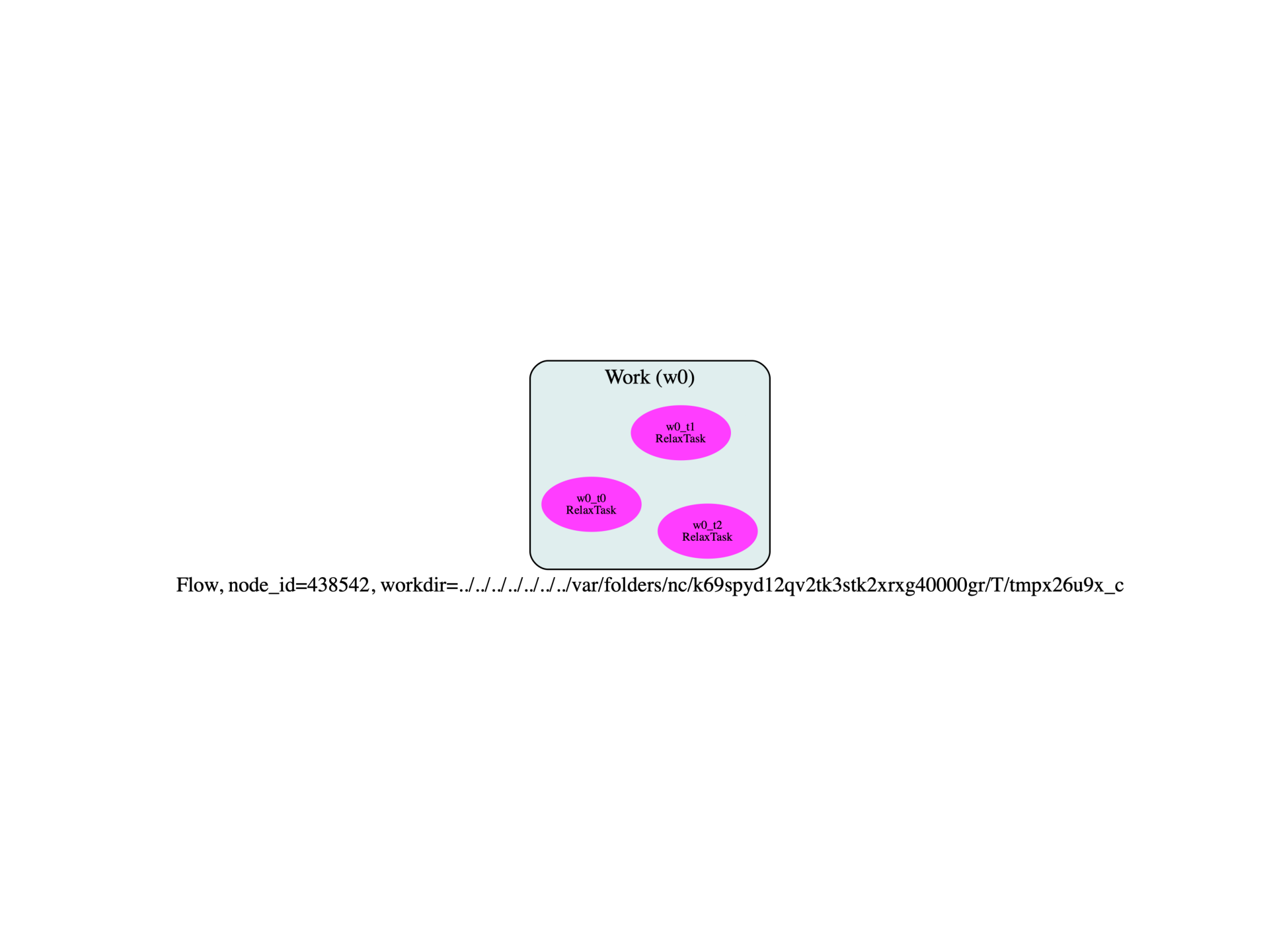
    build_flow(options).graphviz_imshow()


@flowtk.flow_main
def main(options):
    """
    This is our main function that will be invoked by the script.
    flow_main is a decorator implementing the command line interface.
    Command line args are stored in `options`.
    """
    return build_flow(options)


if __name__ == "__main__":
    sys.exit(main())

Run the script with:

run_relax_vs_kpts.py -s

then use:

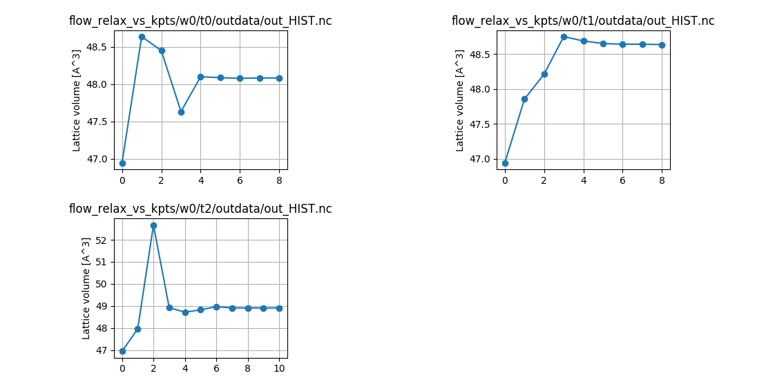
abirun.py flow_relax_vs_kpts hist -p

to print (and plot) the relaxed parameters at the end of the run.

Table with final structures, pressures in GPa and force stats in eV/Ang:

      formula  natom  angle0  angle1  angle2      a      b      c  volume  \
w0_t0  Ga2 N2      4    90.0    90.0   120.0  3.224  3.224  5.343  48.080
w0_t1  Ga2 N2      4    90.0    90.0   120.0  3.249  3.249  5.321  48.635
w0_t2  Ga2 N2      4    90.0    90.0   120.0  3.254  3.254  5.335  48.909

      abispg_num  num_steps  final_energy  final_pressure task_class  \
w0_t0       None          9      -755.344      -1.088e-04  RelaxTask
w0_t1       None          9      -755.632      -5.088e-03  RelaxTask
w0_t2       None         11      -755.645      -4.314e-03  RelaxTask

                                             ncfile              status
w0_t0  flow_relax_vs_kpts/w0/t0/outdata/out_HIST.nc  Completed
w0_t1  flow_relax_vs_kpts/w0/t1/outdata/out_HIST.nc  Completed
w0_t2  flow_relax_vs_kpts/w0/t2/outdata/out_HIST.nc  Completed

The experimental results are:

• Volume of the unit cell of GaN: 45.73 A^3

• Lattice parameters of GaN: a = 3.190 A, c = 5.189 A

• Vertical distance between Ga and N : about 0.377 * c [ Schulz & Thiemann, 1977]