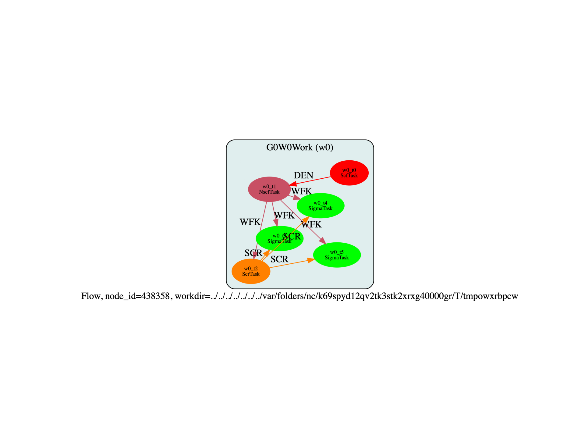
G0W0 flow with convergence study wrt nband

This script shows how to compute the G0W0 corrections in silicon. More specifically, we build a flow to analyze the convergence of the QP corrections wrt to the number of bands in the self-energy. More complicated convergence studies can be implemented on the basis of this example.

import os
import sys

from abipy import abilab, data, flowtk


def make_inputs(ngkpt, paral_kgb=1):
    # Crystalline silicon
    # Calculation of the GW correction to the direct band gap in Gamma
    # Dataset 1: ground state calculation
    # Dataset 2: NSCF calculation
    # Dataset 3: calculation of the screening
    # Dataset 4-5-6: Self-Energy matrix elements (GW corrections) with different values of nband

    multi = abilab.MultiDataset(structure=data.cif_file("si.cif"), pseudos=data.pseudos("14si.pspnc"), ndtset=6)

    # This grid is the most economical, but does not contain the Gamma point.
    scf_kmesh = dict(ngkpt=ngkpt, shiftk=[0.5, 0.5, 0.5, 0.5, 0.0, 0.0, 0.0, 0.5, 0.0, 0.0, 0.0, 0.5])

    # This grid contains the Gamma point, which is the point at which
    # we will compute the (direct) band gap.
    gw_kmesh = dict(ngkpt=ngkpt, shiftk=[0.0, 0.0, 0.0, 0.0, 0.5, 0.5, 0.5, 0.0, 0.5, 0.5, 0.5, 0.0])

    # Global variables. gw_kmesh is used in all datasets except DATASET 1.
    ecut = 6

    multi.set_vars(
        ecut=ecut,
        timopt=-1,
        istwfk="*1",
        paral_kgb=paral_kgb,
        gwpara=2,
    )
    multi.set_kmesh(**gw_kmesh)

    # Dataset 1 (GS run)
    multi[0].set_kmesh(**scf_kmesh)
    multi[0].set_vars(
        tolvrs=1e-6,
        nband=4,
    )

    # Dataset 2 (NSCF run)
    # Here we select the second dataset directly with the syntax multi[1]
    multi[1].set_vars(
        iscf=-2,
        tolwfr=1e-12,
        nband=35,
        nbdbuf=5,
    )

    # Dataset3: Calculation of the screening.
    multi[2].set_vars(
        optdriver=3,
        nband=25,
        ecutwfn=ecut,
        symchi=1,
        inclvkb=0,
        ecuteps=4.0,
        ppmfrq="16.7 eV",
    )

    # Dataset4: Calculation of the Self-Energy matrix elements (GW corrections)
    kptgw = [
        -2.50000000e-01,
        -2.50000000e-01,
        0.00000000e00,
        -2.50000000e-01,
        2.50000000e-01,
        0.00000000e00,
        5.00000000e-01,
        5.00000000e-01,
        0.00000000e00,
        -2.50000000e-01,
        5.00000000e-01,
        2.50000000e-01,
        5.00000000e-01,
        0.00000000e00,
        0.00000000e00,
        0.00000000e00,
        0.00000000e00,
        0.00000000e00,
    ]

    bdgw = [1, 8]

    # Convergence study wrt nband in sigma.
    for idx, nband in enumerate([10, 20, 30]):
        multi[3 + idx].set_vars(
            optdriver=4,
            nband=nband,
            ecutwfn=ecut,
            ecuteps=4.0,
            ecutsigx=6.0,
            symsigma=1,
            # gw_qprange=0,
            # nkptgw=0,
        )
        multi[3 + idx].set_kptgw(kptgw, bdgw)

    return multi.split_datasets()


def build_flow(options):
    # Working directory (default is the name of the script with '.py' removed and "run_" replaced by "flow_")
    if not options.workdir:
        options.workdir = os.path.basename(sys.argv[0]).replace(".py", "").replace("run_", "flow_")

    # Change the value of ngkpt below to perform a GW calculation with a different k-mesh.
    scf, nscf, scr, sig1, sig2, sig3 = make_inputs(ngkpt=[2, 2, 2])

    return flowtk.g0w0_flow(options.workdir, scf, nscf, scr, [sig1, sig2, sig3], manager=options.manager)


# This block generates the thumbnails in the AbiPy gallery.
# You can safely REMOVE this part if you are using this script for production runs.
if os.getenv("READTHEDOCS", False):
    __name__ = None
    import tempfile

    options = flowtk.build_flow_main_parser().parse_args(["-w", tempfile.mkdtemp()])
    build_flow(options).graphviz_imshow()


@flowtk.flow_main
def main(options):
    return build_flow(options)


if __name__ == "__main__":
    sys.exit(main())

Run the script with:

run_si_g0w0.py -s

The last three tasks (w0_t3, w0_t4, w0_t5) are the SigmaTask who have produced a netcdf file with the GW results with different number of bands. We can check this with the command:

abirun.py flow_si_g0w0/ listext SIGRES

Found 3 files with extension `SIGRES` produced by the flow
File                                        Size [Mb]    Node_ID  Node Class
----------------------------------------  -----------  ---------  ------------
flow_si_g0w0/w0/t3/outdata/out_SIGRES.nc         0.05     241325  SigmaTask
flow_si_g0w0/w0/t4/outdata/out_SIGRES.nc         0.08     241326  SigmaTask
flow_si_g0w0/w0/t5/outdata/out_SIGRES.nc         0.13     241327  SigmaTask

Let’s use the SIGRES robot to collect and analyze the results:

abirun.py flow_si_g0w0/ robot SIGRES

and then, inside the ipython terminal, type:

In [1]: df = robot.get_dataframe()
In [2]: df
Out[2]:
                                          nsppol     qpgap            ecutwfn  \
flow_si_g0w0/w0/t3/outdata/out_SIGRES.nc       1  3.627960  5.914381651684836
flow_si_g0w0/w0/t4/outdata/out_SIGRES.nc       1  3.531781  5.914381651684836
flow_si_g0w0/w0/t5/outdata/out_SIGRES.nc       1  3.512285  5.914381651684836

                                                     ecuteps  \
flow_si_g0w0/w0/t3/outdata/out_SIGRES.nc  3.6964885323070074
flow_si_g0w0/w0/t4/outdata/out_SIGRES.nc  3.6964885323070074
flow_si_g0w0/w0/t5/outdata/out_SIGRES.nc  3.6964885323070074

                                                   ecutsigx scr_nband  \
flow_si_g0w0/w0/t3/outdata/out_SIGRES.nc  5.914381651684846        25
flow_si_g0w0/w0/t4/outdata/out_SIGRES.nc  5.914381651684846        25
flow_si_g0w0/w0/t5/outdata/out_SIGRES.nc  5.914381651684846        25

                                         sigma_nband gwcalctyp scissor_ene  \
flow_si_g0w0/w0/t3/outdata/out_SIGRES.nc          10         0         0.0
flow_si_g0w0/w0/t4/outdata/out_SIGRES.nc          20         0         0.0
flow_si_g0w0/w0/t5/outdata/out_SIGRES.nc          30         0         0.0

                                          nkibz
flow_si_g0w0/w0/t3/outdata/out_SIGRES.nc      6
flow_si_g0w0/w0/t4/outdata/out_SIGRES.nc      6
flow_si_g0w0/w0/t5/outdata/out_SIGRES.nc      6

In [3]: %matplotlib
In [4]: df.plot("sigma_nband", "qpgap", marker="o")