Raman with BSE and frozen phonon

This script shows how to perform a Raman calculation with excitonic effects included with the Bethe-Salpeter formalism.

import sys
import os
import numpy as np
import abipy.abilab as abilab
import abipy.data as abidata

from abipy import flowtk


def build_flow(options):
    # Working directory (default is the name of the script with '.py' removed and "run_" replaced by "flow_")
    if not options.workdir:
        options.workdir = os.path.basename(sys.argv[0]).replace(".py", "").replace("run_","flow_")

    flow = flowtk.Flow(options.workdir, manager=options.manager)

    pseudos = abidata.pseudos("14si.pspnc")

    # Get the unperturbed structure.
    base_structure = abidata.structure_from_ucell("Si")

    etas = [-.001, 0, +.001]
    ph_displ = np.reshape(np.zeros(3*len(base_structure)), (-1,3))
    ph_displ[0,:] = [+1, 0, 0]
    ph_displ[1,:] = [-1, 0, 0]

    # Build new structures by displacing atoms according to the phonon displacement
    # ph_displ (in cartesian coordinates). The Displacement is normalized so that
    # the maximum atomic diplacement is 1 Angstrom and then multiplied by eta.
    modifier = abilab.StructureModifier(base_structure)

    displaced_structures = modifier.displace(ph_displ, etas, frac_coords=False)

    # Generate the different shifts to average
    ndiv = 2
    shift1D = np.arange(1,2*ndiv+1,2)/(2*ndiv)
    all_shifts = [[x,y,z] for x in shift1D for y in shift1D for z in shift1D]
    all_shifts = [[0, 0, 0]]

    for structure, eta in zip(displaced_structures, etas):
        for shift in all_shifts:
            flow.register_work(raman_work(structure, pseudos, shift))

    return flow


def raman_work(structure, pseudos, shiftk, paral_kgb=1):
    # Generate 3 different input files for computing optical properties with BSE.

    # Global variables
    global_vars = dict(
        ecut=8,
        istwfk="*1",
        chksymbreak=0,
        #nstep=4,
        nstep=10,
        paral_kgb=paral_kgb,
    )

    # GS run
    scf_inp = abilab.AbinitInput(structure, pseudos=pseudos)
    scf_inp.set_vars(global_vars)
    scf_inp.set_kmesh(ngkpt=[2, 2, 2], shiftk=shiftk)
    scf_inp["tolvrs"] = 1e-6

    # NSCF run
    nscf_inp = abilab.AbinitInput(structure, pseudos=pseudos)
    nscf_inp.set_vars(global_vars)
    nscf_inp.set_kmesh(ngkpt=[2, 2, 2], shiftk=shiftk)

    nscf_inp.set_vars(
        tolwfr=1e-8,
        nband=12,
        nbdbuf=4,
        iscf=-2,
    )

    # BSE run with Model dielectric function and Haydock (only resonant + W + v)
    # Note that SCR file is not needed here
    bse_inp = abilab.AbinitInput(structure, pseudos=pseudos)
    bse_inp.set_vars(global_vars)
    bse_inp.set_kmesh(ngkpt=[2, 2, 2], shiftk=shiftk)

    bse_inp.set_vars(
        optdriver=99,
        ecutwfn=global_vars["ecut"],
        ecuteps=3,
        inclvkb=2,
        bs_algorithm=2,       # Haydock
        bs_haydock_niter=4,   # No. of iterations for Haydock
        bs_exchange_term=1,
        bs_coulomb_term=21,   # Use model W and full W_GG.
        mdf_epsinf=12.0,
        bs_calctype=1,        # Use KS energies and orbitals to construct L0
        mbpt_sciss="0.8 eV",
        bs_coupling=0,
        bs_loband=2,
        nband=6,
        #bs_freq_mesh="0 10 0.1 eV",
        bs_hayd_term=0,      # No terminator
    )

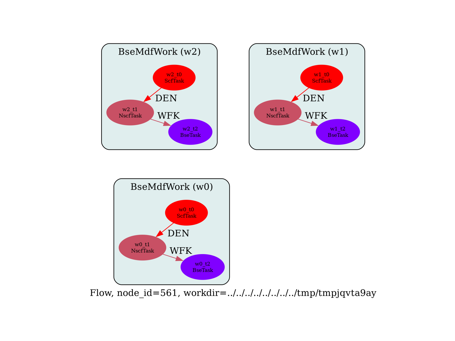
    # Build the work representing a BSE run with model dielectric function.
    return flowtk.BseMdfWork(scf_inp, nscf_inp, bse_inp)


# This block generates the thumbnails in the AbiPy gallery.
# You can safely REMOVE this part if you are using this script for production runs.
if os.getenv("READTHEDOCS", False):
    __name__ = None
    import tempfile
    options = flowtk.build_flow_main_parser().parse_args(["-w", tempfile.mkdtemp()])
    build_flow(options).graphviz_imshow()


@flowtk.flow_main
def main(options):
    """
    This is our main function that will be invoked by the script.
    flow_main is a decorator implementing the command line interface.
    Command line args are stored in `options`.
    """
    return build_flow(options)


if __name__ == "__main__":
    sys.exit(main())

Run the script with:

run_raman_bse.py -s

then use:

abirun.py flow_raman_bse robot MDF

to analyze all the macroscopic dielectric functions produced by the Flow with the robot. Inside the ipython terminal type:

[1] %matplotlib
[2] robot.plot()

to compare the real and imaginary part of the macroscopic dielectric function for the different displacements.