Born effective charges and dielectric tensors with DFPT

This example shows how to compute the Born effective charges and the dielectric tensors (e0, einf) of AlAs with AbiPy flows. We perform multiple calculations by varying the number of k-points in order to analyze the convergence of the results wrt nkpt.

import sys
import os
import abipy.abilab as abilab
import abipy.data as abidata

from abipy import flowtk


def make_scf_input(ngkpt, paral_kgb=0):
    """
    This function constructs the input file for the GS calculation for a given IBZ sampling.
    """
    # Crystalline AlAs: computation of the second derivative of the total energy
    structure = abidata.structure_from_ucell("AlAs")
    pseudos = abidata.pseudos("13al.981214.fhi", "33as.pspnc")
    gs_inp = abilab.AbinitInput(structure, pseudos=pseudos)

    gs_inp.set_vars(
        nband=4,
        ecut=2.0,
        ngkpt=ngkpt,
        nshiftk=4,
        shiftk=[0.0, 0.0, 0.5,   # This gives the usual fcc Monkhorst-Pack grid
                0.0, 0.5, 0.0,
                0.5, 0.0, 0.0,
                0.5, 0.5, 0.5],
        #shiftk=[0, 0, 0],
        paral_kgb=paral_kgb,
        tolvrs=1.0e-10,
        diemac=9.0,
        ixc=1,      # This is needed because the pseudos have been generated with different XC
        #iomode=3,
    )

    return gs_inp


def build_flow(options):
    """
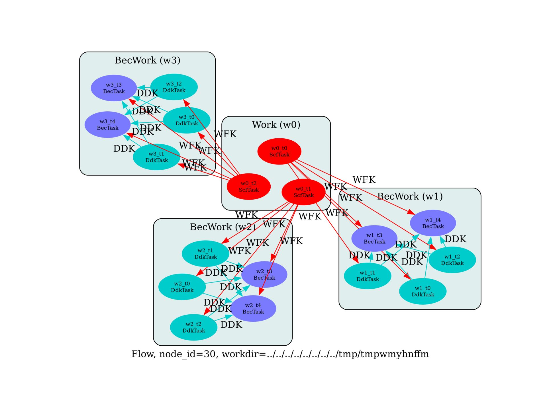
    Create a `Flow` for phonon calculations. The flow has two works.

    The first work contains a single GS task that produces the WFK file used in DFPT
    Then we have multiple Works that are generated automatically
    in order to compute the dynamical matrix on a [4, 4, 4] mesh.
    Symmetries are taken into account: only q-points in the IBZ are generated and
    for each q-point only the independent atomic perturbations are computed.
    """
    # Working directory (default is the name of the script with '.py' removed and "run_" replaced by "flow_")
    if not options.workdir:
        options.workdir = os.path.basename(sys.argv[0]).replace(".py", "").replace("run_", "flow_")

    flow = flowtk.Flow(workdir=options.workdir)

    for ngkpt in [(2, 2, 2), (4, 4, 4), (8, 8, 8)]:
        # Build input for GS calculation with different k-meshes
        scf_input = make_scf_input(ngkpt=ngkpt)
        flow.register_scf_task(scf_input, append=True)

    for scf_task in flow[0]:
        bec_work = flowtk.BecWork.from_scf_task(scf_task)
        flow.register_work(bec_work)

    return flow


# This block generates the thumbnails in the AbiPy gallery.
# You can safely REMOVE this part if you are using this script for production runs.
if os.getenv("READTHEDOCS", False):
    __name__ = None
    import tempfile
    options = flowtk.build_flow_main_parser().parse_args(["-w", tempfile.mkdtemp()])
    build_flow(options).graphviz_imshow()


@flowtk.flow_main
def main(options):
    """
    This is our main function that will be invoked by the script.
    flow_main is a decorator implementing the command line interface.
    Command line args are stored in `options`.
    """
    return build_flow(options)


if __name__ == "__main__":
    sys.exit(main())

Run the script with:

run_becs_and_epsilon_vs_kpts.py -s

Use:

abirun.py flow_becs_and_epsilon_vs_kpts/ listext DDB

to list all the DDB files produced by the flow.

Now use abicomp.py to create a DdbRobot to analyze the DDB files produced by the 3 Works:

abicomp.py ddb flow_becs_and_epsilon_vs_kpts/w*/outdata/out_DDB

the inside the ipython terminal use the anacompare methods to analyze the results. e.g.

In [1]: r = robot.anacompare_epsinf()
In [2]: r.df
Out[2]:
          xx         yy         zz   yz   xz   xy  formula  chneut  \
0  13.584082  13.584082  13.584082  0.0  0.0  0.0  Al1 As1       1
0   9.268425   9.268425   9.268425  0.0  0.0  0.0  Al1 As1       1
0   8.873178   8.873178   8.873178  0.0  0.0  0.0  Al1 As1       1