e-ph scattering potentials

This example shows how to compute e-ph scattering potentials along a q-path, merge the POT files in the DVDB file and finally use the DVDB and the DDB file to analyze the average over the unit cell of the periodic part as a function of q

import sys
import os
import abipy.abilab as abilab
import abipy.data as abidata

from abipy import flowtk


def make_scf_input(ngkpt):
    """
    This function constructs the input file for the GS calculation:
    """
    structure = dict(
        angdeg=3*[60.0],
        acell=3*[7.1992351952],
        natom=2,
        ntypat=2,
        typat=[1, 2],
        znucl=[31, 15],
        xred=[
            0.0000000000, 0.0000000000, 0.0000000000,
            0.2500000000, 0.2500000000, 0.2500000000,
        ])

    pseudos = abidata.pseudos("Ga.oncvpsp", "P.psp8")
    gs_inp = abilab.AbinitInput(structure, pseudos=pseudos)

    gs_inp.set_vars(
        nband=8,
        ecut=20.0,   # Too low
        ngkpt=ngkpt,
        nshiftk=1,
        shiftk=[0, 0, 0],
        tolvrs=1.0e-8,
        nstep=150,
        paral_kgb=0,
    )

    return gs_inp


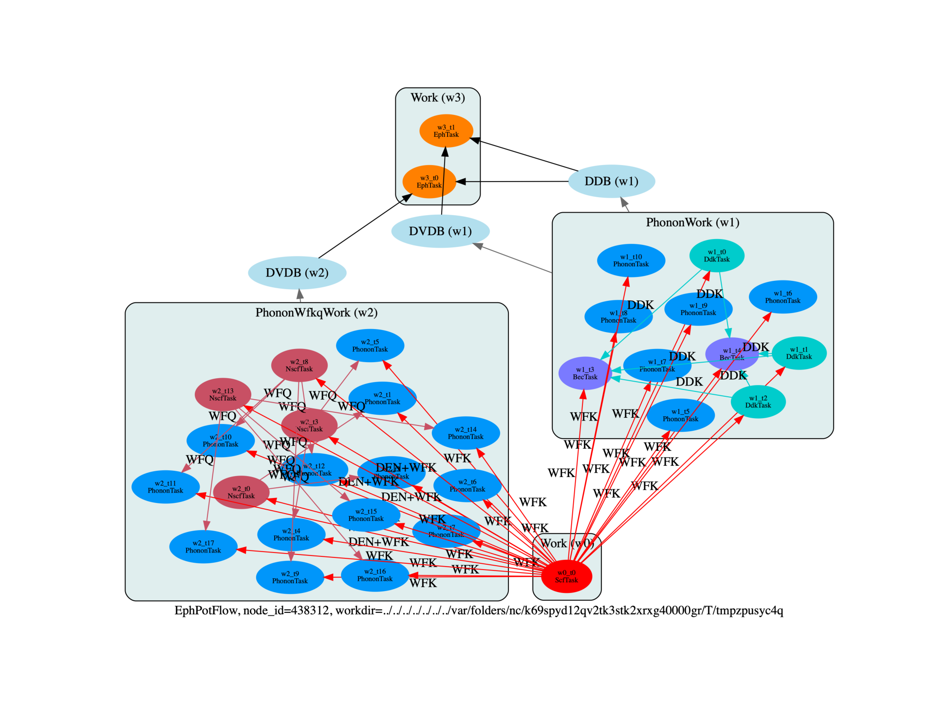
def build_flow(options):
    """
    Create a `Flow` for phonon calculations. The flow has two works.

    The first work contains a single GS task that produces the WFK file used in DFPT
    Then we have multiple Works that are generated automatically
    in order to compute the dynamical matrix on a [2, 2, 2] mesh.
    Symmetries are taken into account: only q-points in the IBZ are generated and
    for each q-point only the independent atomic perturbations are computed.
    """
    # Working directory (default is the name of the script with '.py' removed and "run_" replaced by "flow_")
    if not options.workdir:
        options.workdir = os.path.basename(sys.argv[0]).replace(".py", "").replace("run_", "flow_")

    # Use 2x2x2 both for k-mesh and q-mesh
    # Build input for GS calculation
    scf_input = make_scf_input(ngkpt=(2, 2, 2))

    # Create flow to compute all the independent atomic perturbations
    # corresponding to a [4, 4, 4] q-mesh.
    # Electric field and Born effective charges are also computed.
    from abipy.flowtk.eph_flows import EphPotFlow
    ngqpt = [2, 2, 2]

    qpath_list = [
        +0.10000,  +0.10000,  +0.10000,  # L -> G
        +0.00000,  +0.00000,  +0.00000,  # $\Gamma$
        +0.10000,  +0.00000,  +0.10000,  # G -> X

        #+0.50000,  +0.50000,  +0.50000,  # L
        #+0.00000,  +0.00000,  +0.00000,  # $\Gamma$
        #+0.50000,  +0.00000,  +0.50000,  # X
        #+0.50000,  +0.25000,  +0.75000,  # W
        #+0.37500,  +0.37500,  +0.75000,  # K
        #+0.00000,  +0.00000,  +0.00000,  # $\Gamma$
        #+0.50000,  +0.25000,  +0.75000,  # W
        #+0.62500  +0.25000  +0.62500  # U
        #+0.50000  +0.25000  +0.75000  # W
        #+0.50000  +0.50000  +0.50000  # L
        #+0.37500  +0.37500  +0.75000  # K
        #+0.62500  +0.25000  +0.62500  # U
        #+0.50000  +0.00000  +0.50000  # X
    ]

    # Use small ndivsm to reduce computing time.
    flow = EphPotFlow.from_scf_input(options.workdir, scf_input,
                                     ngqpt, qpath_list, ndivsm=2, ddk_tolerance={"tolwfr": 1e-12},
                                     with_becs=True, with_quad=False)

    return flow


# This block generates the thumbnails in the Abipy gallery.
# You can safely REMOVE this part if you are using this script for production runs.
if os.getenv("READTHEDOCS", False):
    __name__ = None
    import tempfile
    options = flowtk.build_flow_main_parser().parse_args(["-w", tempfile.mkdtemp()])
    build_flow(options).graphviz_imshow()


@flowtk.flow_main
def main(options):
    """
    This is our main function that will be invoked by the script.
    flow_main is a decorator implementing the command line interface.
    Command line args are stored in `options`.
    """
    return build_flow(options)


if __name__ == "__main__":
    sys.exit(main())