Band structure with/without SOC

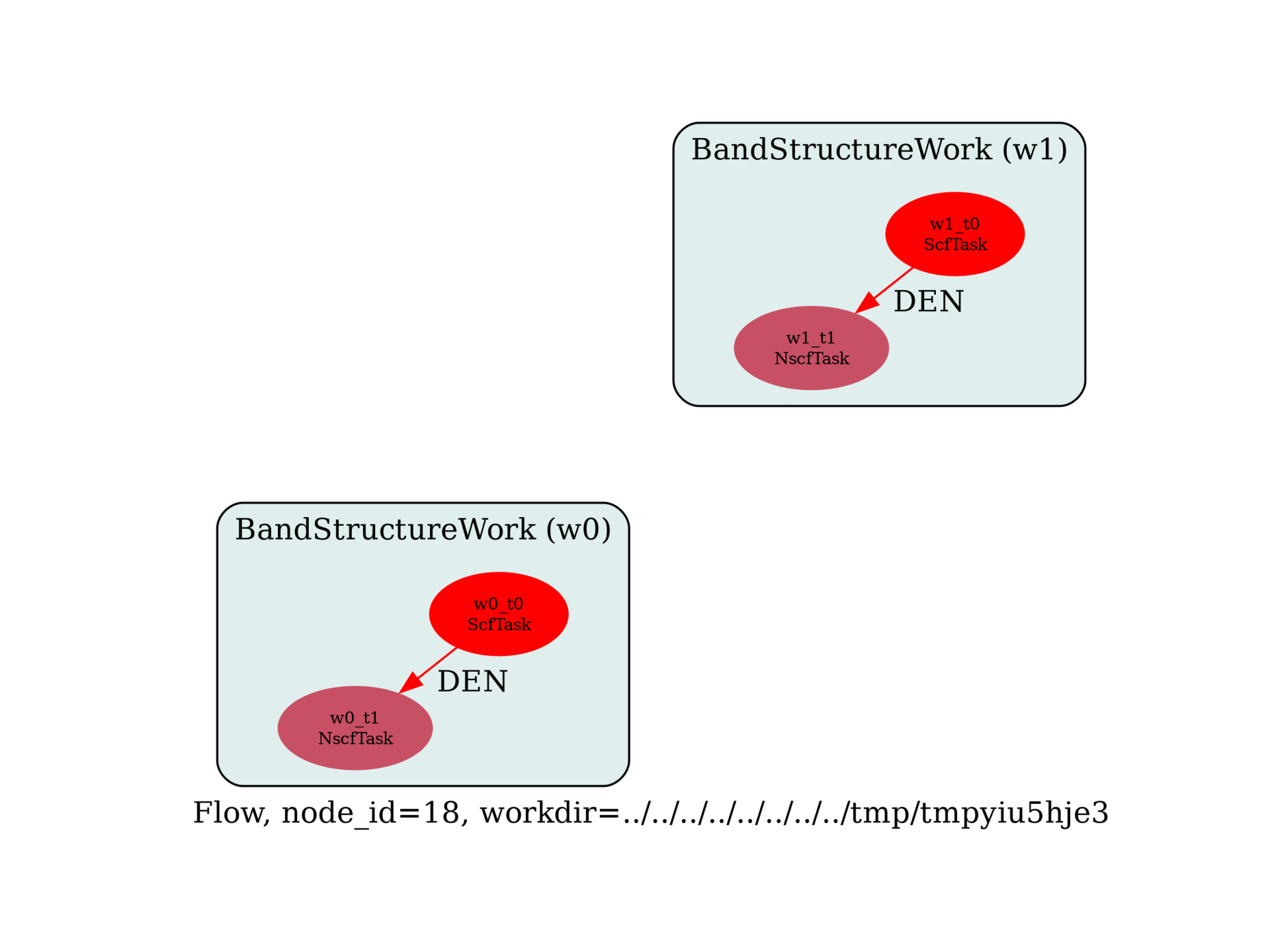
This example shows how to compute the band structure of GaAs with and without spin-orbit term. We essentially build two BandStructureWork inside a loop over nspinor in [1, 2] nspinor = 1 corresponds to a standard collinear calculation for non-magnetic systems while nspinor = 2 gives us the non-collinear case with spinor wavefunctions required for the treatment of SOC. Some of the variables in the input files must be changed depending on the value of nspinor.

We use relativistic NC pseudos made of two terms: scalar pseudo + SOC term. The SOC term can be deactivated with the input variable so_psp.

import sys
import os
import abipy.data as abidata
import abipy.abilab as abilab
import abipy.flowtk as flowtk


def build_flow(options):
    # Set working directory (default is the name of the script with '.py' removed and "run_" replaced by "flow_")
    if not options.workdir:
        options.workdir = os.path.basename(sys.argv[0]).replace(".py", "").replace("run_", "flow_")

    structure = abidata.structure_from_ucell("GaAs")
    pseudos = abidata.pseudos("Ga-low_r.psp8", "As_r.psp8")
    num_electrons = structure.num_valence_electrons(pseudos)
    #print("num_electrons:", num_electrons)

    # Usa same shifts in all tasks.
    ngkpt = [4, 4, 4]
    shiftk = [
        [0.5, 0.5, 0.5],
        [0.5, 0.0, 0.0],
        [0.0, 0.5, 0.0],
        [0.0, 0.0, 0.5],
    ]

    # NSCF run on k-path with large number of bands
    kptbounds = [
        [0.5, 0.0, 0.0],  # L point
        [0.0, 0.0, 0.0],  # Gamma point
        [0.0, 0.5, 0.5],  # X point
    ]

    # Initialize the flow.
    flow = flowtk.Flow(options.workdir, manager=options.manager)

    for nspinor in [1, 2]:
        # Multi will contain two datasets (GS + NSCF) for the given nspinor.
        multi = abilab.MultiDataset(structure=structure, pseudos=pseudos, ndtset=2)

        # Global variables.
        multi.set_vars(
            ecut=20,
            nspinor=nspinor,
            nspden=1 if nspinor == 1 else 4,
            so_psp="*0" if nspinor == 1 else "*1",   # Important!
            #paral_kgb=1,
        )

        nband_occ = num_electrons // 2 if nspinor == 1 else num_electrons
        #print(nband_occ)

        # Dataset 1 (GS run)
        multi[0].set_vars(tolvrs=1e-8, nband=nband_occ + 4)
        multi[0].set_kmesh(ngkpt=ngkpt, shiftk=shiftk, kptopt=1 if nspinor == 1 else 4)

        multi[1].set_vars(iscf=-2, nband=nband_occ + 4, tolwfr=1.e-12)
        multi[1].set_kpath(ndivsm=10, kptbounds=kptbounds)

        # Get the SCF and the NSCF input.
        scf_input, nscf_input = multi.split_datasets()

        flow.register_work(flowtk.BandStructureWork(scf_input, nscf_input))

    return flow


# This block generates the thumbnails in the AbiPy gallery.
# You can safely REMOVE this part if you are using this script for production runs.
if os.getenv("READTHEDOCS", False):
    __name__ = None
    import tempfile
    options = flowtk.build_flow_main_parser().parse_args(["-w", tempfile.mkdtemp()])
    build_flow(options).graphviz_imshow()


@flowtk.flow_main
def main(options):
    """
    This is our main function that will be invoked by the script.
    flow_main is a decorator implementing the command line interface.
    Command line args are stored in `options`.
    """
    return build_flow(options)


if __name__ == "__main__":
    sys.exit(main())

Run the script with:

run_gaas_ebands_soc.py -s

then use:

abirun.py flow_si_ebands ebands –plot -t NscfTask

to analyze (and plot) the electronic bands produced by the NsfTasks of the Flow.

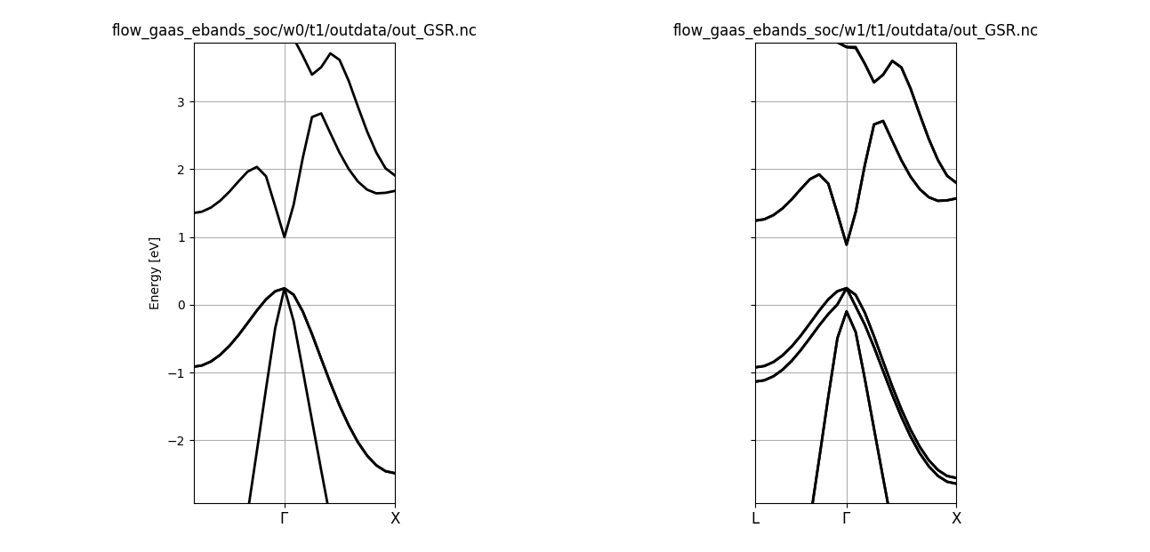
Alternatively, one can start a GSR robot for the NscfTask with:

abirun.py flow_gaas_ebands_soc/ robot GSR -t NscfTask

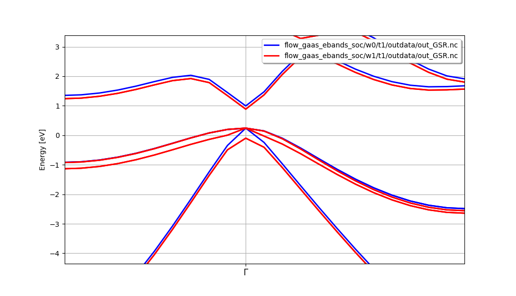
and then plot the two band structure on the same figure with:

In [1]: %matplotlib
In [2]: robot.combiplot_ebands()