Convergence studies of e-DOS wrt ngkpt

This examples shows how to build a Flow to compute the band structure and the electron DOS of MgB2 with different k-point samplings.

import os
import sys
import abipy.data as abidata
import abipy.abilab as abilab
from abipy import flowtk


def make_scf_nscf_inputs(structure, pseudos, paral_kgb=1):
    """return GS, NSCF (band structure), and DOSes input."""

    multi = abilab.MultiDataset(structure, pseudos=pseudos, ndtset=5)

    # Global variables
    multi.set_vars(
        ecut=10,
        nband=11,
        timopt=-1,
        occopt=4,    # Marzari smearing
        tsmear=0.03,
        paral_kgb=paral_kgb,
   )

    # Dataset 1 (GS run)
    multi[0].set_kmesh(ngkpt=[8, 8, 8], shiftk=structure.calc_shiftk())
    multi[0].set_vars(tolvrs=1e-6)

    # Dataset 2 (NSCF Band Structure)
    multi[1].set_kpath(ndivsm=6)
    multi[1].set_vars(tolwfr=1e-12)

    # Dos calculations with increasing k-point sampling.
    for i, nksmall in enumerate([4, 8, 16]):
        multi[i+2].set_vars(
            iscf=-3,   # NSCF calculation
            ngkpt=structure.calc_ngkpt(nksmall),
            shiftk=[0.0, 0.0, 0.0],
            tolwfr=1.0e-10,
        )

    # return GS, NSCF (band structure), DOSes input.
    return multi.split_datasets()


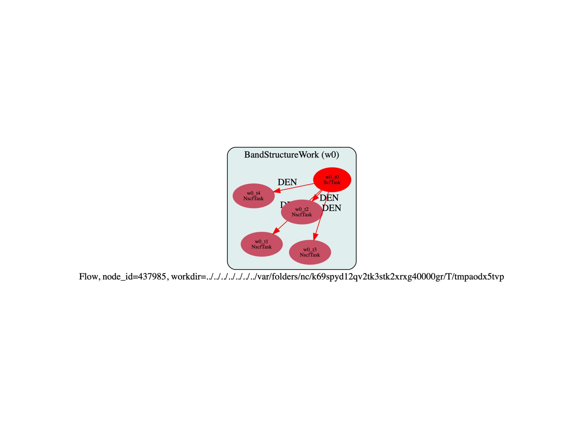
def build_flow(options):
    # Working directory (default is the name of the script with '.py' removed and "run_" replaced by "flow_")
    if not options.workdir:
        options.workdir = os.path.basename(sys.argv[0]).replace(".py", "").replace("run_", "flow_")

    structure = abidata.structure_from_ucell("MgB2")

    # Get pseudos from a table.
    table = abilab.PseudoTable(abidata.pseudos("12mg.pspnc", "5b.pspnc"))
    pseudos = table.get_pseudos_for_structure(structure)

    inputs = make_scf_nscf_inputs(structure, pseudos)
    scf_input, nscf_input, dos_inputs = inputs[0], inputs[1], inputs[2:]

    return flowtk.bandstructure_flow(options.workdir, scf_input, nscf_input,
                                     dos_inputs=dos_inputs, manager=options.manager)


# This block generates the thumbnails in the AbiPy gallery.
# You can safely REMOVE this part if you are using this script for production runs.
if os.getenv("READTHEDOCS", False):
    __name__ = None
    import tempfile
    options = flowtk.build_flow_main_parser().parse_args(["-w", tempfile.mkdtemp()])
    build_flow(options).graphviz_imshow()


@flowtk.flow_main
def main(options):
    """
    This is our main function that will be invoked by the script.
    flow_main is a decorator implementing the command line interface.
    Command line args are stored in `options`.
    """
    return build_flow(options)


if __name__ == "__main__":
    sys.exit(main())

Run the script with:

run_mgb2_edoses.py -s

then use:

abirun.py flow_mgb2_edoes ebands

to get info about the electronic properties:

KS electronic bands:
       nsppol  nspinor  nspden  nkpt  nband  nelect  fermie formula  natom  \
w0_t0       1        1       1    40     11     8.0   7.615  Mg1 B2      3
w0_t1       1        1       1    97     11     8.0   7.615  Mg1 B2      3
w0_t2       1        1       1    15     11     8.0   7.701  Mg1 B2      3
w0_t3       1        1       1    80     11     8.0   7.629  Mg1 B2      3
w0_t4       1        1       1   432     11     8.0   7.626  Mg1 B2      3

       angle0  angle1  angle2      a      b      c  volume abispg_num  \
w0_t0    90.0    90.0   120.0  3.086  3.086  3.523  29.056        191
w0_t1    90.0    90.0   120.0  3.086  3.086  3.523  29.056        191
w0_t2    90.0    90.0   120.0  3.086  3.086  3.523  29.056        191
w0_t3    90.0    90.0   120.0  3.086  3.086  3.523  29.056        191
w0_t4    90.0    90.0   120.0  3.086  3.086  3.523  29.056        191

                                                  scheme  occopt  tsmear_ev  \
w0_t0  cold smearing of N. Marzari with minimization ...       4      0.816
w0_t1  cold smearing of N. Marzari with minimization ...       4      0.816
w0_t2  cold smearing of N. Marzari with minimization ...       4      0.816
w0_t3  cold smearing of N. Marzari with minimization ...       4      0.816
w0_t4  cold smearing of N. Marzari with minimization ...       4      0.816

       bandwidth_spin0  fundgap_spin0  dirgap_spin0 task_class  \
w0_t0           12.452          0.031         0.609    ScfTask
w0_t1           12.441          0.077         0.399   NscfTask
w0_t2           12.368          0.415         1.680   NscfTask
w0_t3           12.510          0.069         0.390   NscfTask
w0_t4           12.506          0.033         0.283   NscfTask

                                          ncfile  node_id              status
w0_t0  flow_mgb2_edoses/w0/t0/outdata/out_GSR.nc   241032  Completed
w0_t1  flow_mgb2_edoses/w0/t1/outdata/out_GSR.nc   241033  Completed
w0_t2  flow_mgb2_edoses/w0/t2/outdata/out_GSR.nc   241034  Completed
w0_t3  flow_mgb2_edoses/w0/t3/outdata/out_GSR.nc   241035  Completed
w0_t4  flow_mgb2_edoses/w0/t4/outdata/out_GSR.nc   241036  Completed

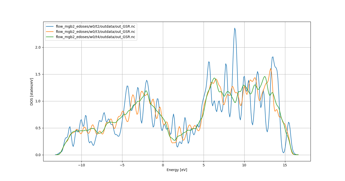
Our main goal is to analyze the convergence of the DOS wrt to the k-point sampling. As we know that w0_t2, w0_t3` and w0_t4 are DOS calculations, we can build a GSR robot for these tasks with:

abirun.py flow_mgb2_edoses/ ebands -nids=241034,241035,241036

then, inside the ipython shell, one can use:

In [1]: %matplotlib
In [2]: robot.combiplot_edos()

to plot the electronic DOS obtained with different number of k-points in the IBZ.