Optic Flow

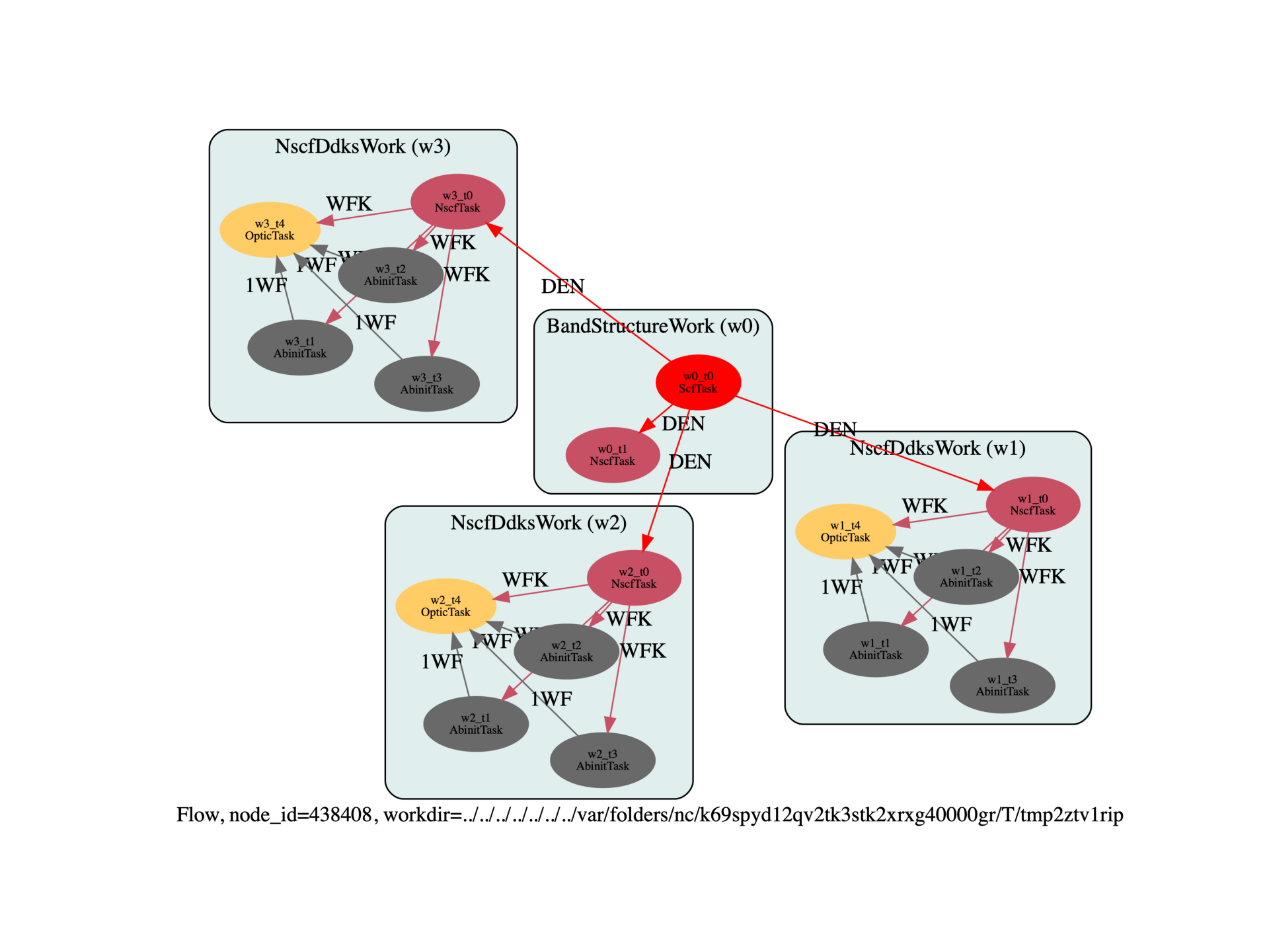
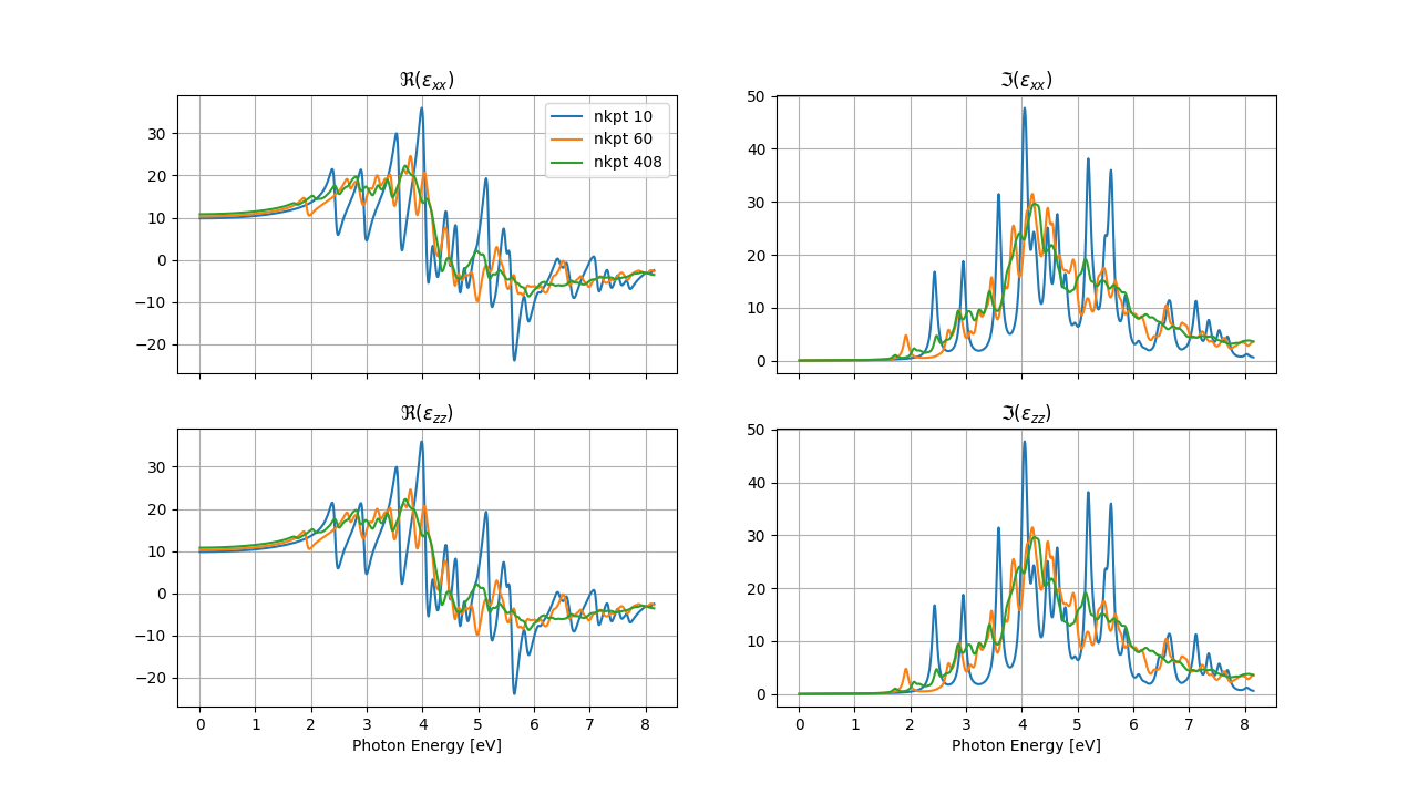
This example shows how to create a Flow to compute optical spectra with Optic (independent particle approximation, no local field effects) and perform a convergence study with respect to the k-point sampling.

import sys
import os
import abipy.data as abidata
import abipy.abilab as abilab
import abipy.flowtk as flowtk


def build_flow(options, paral_kgb=0):
    """
    Build flow for the calculation of optical properties with optic + band structure
    along high-symmetry k-path. DDK are computed with 3 k-meshes of increasing density
    to monitor the convergece of the spectra.
    """
    # Working directory (default is the name of the script with '.py' removed and "run_" replaced by "flow_")
    if not options.workdir:
        options.workdir = os.path.basename(sys.argv[0]).replace(".py", "").replace("run_", "flow_")

    multi = abilab.MultiDataset(structure=abidata.structure_from_ucell("GaAs"),
                                pseudos=abidata.pseudos("31ga.pspnc", "33as.pspnc"), ndtset=2)

    # Usa same shifts in all tasks.
    shiftk = [[0.5, 0.5, 0.5],
              [0.5, 0.0, 0.0],
              [0.0, 0.5, 0.0],
              [0.0, 0.0, 0.5]]

    # Global variables.
    multi.set_vars(ecut=2, paral_kgb=paral_kgb)

    # Dataset 1 (GS run)
    multi[0].set_vars(tolvrs=1e-8, nband=4)
    multi[0].set_kmesh(ngkpt=[4, 4, 4], shiftk=shiftk)

    # NSCF run on k-path with large number of bands
    multi[1].set_vars(iscf=-2, nband=20, tolwfr=1.e-9)
    multi[1].set_kpath(ndivsm=10)

    # Initialize the flow.
    flow = flowtk.Flow(options.workdir, manager=options.manager)

    # GS to get the density + NSCF along the path.
    scf_inp, nscf_inp = multi.split_datasets()
    bands_work = flowtk.BandStructureWork(scf_inp, nscf_inp)
    flow.register_work(bands_work)

    # Build OpticInput used to compute optical properties.
    optic_input = abilab.OpticInput(
        broadening=0.002,          # Value of the smearing factor, in Hartree
        domega=0.0003,             # Frequency mesh.
        maxomega=0.3,
        scissor=0.000,             # Scissor shift if needed, in Hartree
        tolerance=0.002,           # Tolerance on closeness of singularities (in Hartree)
        num_lin_comp=2,            # Number of components of linear optic tensor to be computed
        lin_comp=(11, 33),         # Linear coefficients to be computed (x=1, y=2, z=3)
        num_nonlin_comp=2,         # Number of components of nonlinear optic tensor to be computed
        nonlin_comp=(123, 222),    # Non-linear coefficients to be computed
    )

    # ddk_nband is fixed here, in principle it depends on nelect and the frequency range in chi(w).
    ddk_nband = 20

    # Perform converge study wrt ngkpt (shiftk is constant).
    ngkpt_convergence = [[4, 4, 4], [8, 8, 8], [16, 16, 16]]

    from abipy.flowtk.dfpt_works import NscfDdksWork
    for ddk_ngkpt in ngkpt_convergence:
        # Build work for NSCF from DEN produced by the first GS task + 3 DDKs.
        # All tasks use more bands and a denser k-mesh defined by ddk_ngkpt.
        ddks_work = NscfDdksWork.from_scf_task(bands_work[0], ddk_ngkpt, shiftk, ddk_nband)
        flow.register_work(ddks_work)

        # Build optic task to compute chi with this value of ddk_ngkpt.
        optic_task = flowtk.OpticTask(optic_input, nscf_node=ddks_work.task_with_ks_energies,
                                      ddk_nodes=ddks_work.ddk_tasks, use_ddknc=False)
        ddks_work.register_task(optic_task)

    return flow


# This block generates the thumbnails in the AbiPy gallery.
# You can safely REMOVE this part if you are using this script for production runs.
if os.getenv("READTHEDOCS", False):
    __name__ = None
    import tempfile
    options = flowtk.build_flow_main_parser().parse_args(["-w", tempfile.mkdtemp()])
    build_flow(options).graphviz_imshow()


@flowtk.flow_main
def main(options):
    """
    This is our main function that will be invoked by the script.
    flow_main is a decorator implementing the command line interface.
    Command line args are stored in `options`.
    """
    return build_flow(options)


if __name__ == "__main__":
    sys.exit(main())

Run the script with:

run_optic.py -s

then use:

abirun.py flow_optic robot optic

to create a robot for OPTIC.nc files. Then inside the ipytho shell type:

In [1]: %matplotlib
In [2]: robot.plot_linopt_convergence()