Screening computation with different parameters

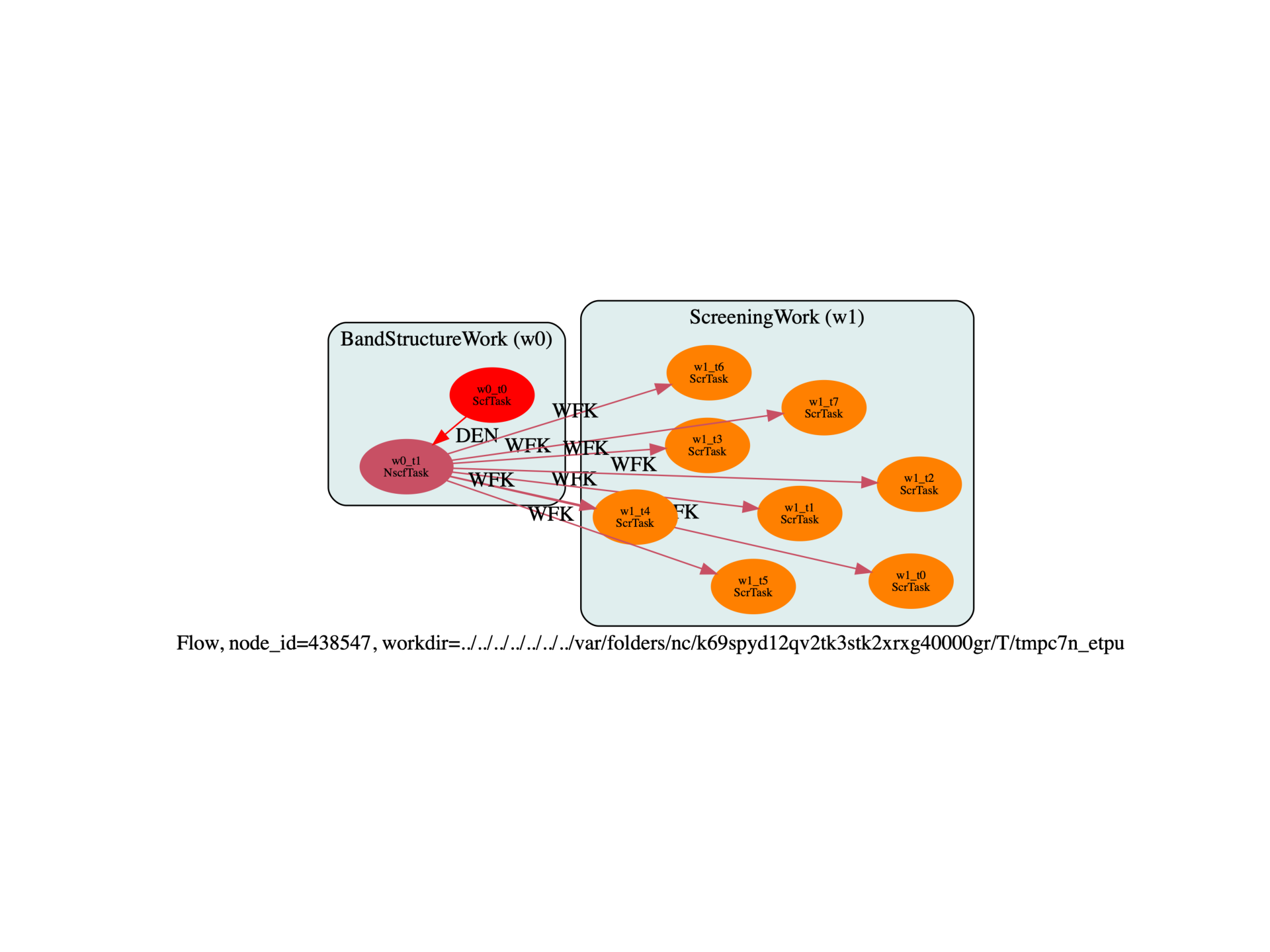
This examples shows how to compute the SCR file with different number of bands and different values of ecuteps in order to prepare further GW convergence studies. Each screening calculation is automatically parallelized over q-points and the partial SCR files are then merged with the mrgscr utility. The total SCR file is available in the outdata directory of the ScreeningWork.

Number of valence electrons in the unit cell: 8

import sys
import os
import numpy as np

import abipy.abilab as abilab
import abipy.data as abidata
import abipy.flowtk as flowtk


def build_flow(options):

    # Working directory (default is the name of the script with '.py' removed and "run_" replaced by "flow_")
    if not options.workdir:
        options.workdir = os.path.basename(sys.argv[0]).replace(".py", "").replace("run_", "flow_")


    # Initialize structure from string and a minimalistic variables:
    # natom, acell, rprimd and xred_symbols.

    structure = abilab.Structure.from_abistring("""
natom 2
acell  3*10.26         # Experimental lattice constants
rprim  0.0  0.5  0.5   # FCC primitive vectors (to be scaled by acell)
       0.5  0.0  0.5
       0.5  0.5  0.0

xred_symbols
      0.0  0.0  0.0  Si
      0.25 0.25 0.25 Si
""")

    # Build the SCF input.
    scf_inp = abilab.AbinitInput(structure=structure, pseudos=abidata.pseudos("14si.pspnc"))

    #nscf_nband_list = np.arange(2, 8, 2)
    nscf_nband_list = [25]
    max_nscf_nband = max(nscf_nband_list)

    #ecuteps_list = np.arange(2, 8, 2)
    ecuteps_list = [2]
    max_ecuteps = max(ecuteps_list)

    print("Number of valence electrons in the unit cell:", scf_inp.num_valence_electrons)

    scf_inp.set_vars(
        ecut=4,
        nband=8,
        ngkpt=[4, 4, 4],
        shiftk=[0, 0, 0],
        tolvrs=1e-8,
        timopt=-1,   # TODO: Add abirun.py option to extract timing data.
        #paral_kgb=1,
        #iomode=3,
    )

    #ebands_inp = scf_inp.make_ebands_input(ndivsm=15)

    # Build NSCF input on a k-mesh including empty states.
    nscf_inp = scf_inp.new_with_vars(
        nband=max_nscf_nband,
        #nbdbuf=10
        tolwfr=1e-20,   # Too high. Should be ~1e-20
        iscf=-2
    )

    flow = flowtk.Flow(workdir=options.workdir, manager=options.manager)

    # Band structure work to produce the WFK file with a NSCF run + empty states.
    bands_work = flowtk.BandStructureWork(scf_inp, nscf_inp) # dos_inputs=[nscf_inp])
    flow.register_work(bands_work)

    for ecuteps in ecuteps_list:
        for nscf_nband in nscf_nband_list:

            scr_inp = nscf_inp.new_with_vars(
                optdriver=3,
                ecuteps=ecuteps,
                nband=nscf_nband,
            )

            # Compute SCR file by splitting all the q-points.
            scr_work = flowtk.ScreeningWork.from_nscf_task(bands_work.nscf_task, scr_inp)

            # IMPORTANT:
            #   If you alredy have a WFK file and you want to skip the SCF + NSCF part
            #   build the scr_work using `from_wkf_filepath` instead of `from_nscf_task` e.g.:

            #scr_work = ScreeningWork.from_wfk_file(wfk_filepath, scr_inp)

            flow.register_work(scr_work)

            # This part is optional:
            #     1) set_readme sets the string that will be used to generate a human readable README.md file
            #     2) set_abipy_meta_json can be used to defined metadata that will be written to abipy_meta.json.
            scr_work.set_readme(f"SCR computation with ecuteps={ecuteps} and nband={nscf_nband}")
            scr_work.set_abipy_meta_json(dict(ecuteps=ecuteps, nband=nscf_nband))

    return flow


# This block generates the thumbnails in the AbiPy gallery.
# You can safely REMOVE this part if you are using this script for production runs.
if os.getenv("READTHEDOCS", False):
    __name__ = None
    import tempfile
    options = flowtk.build_flow_main_parser().parse_args(["-w", tempfile.mkdtemp()])
    build_flow(options).graphviz_imshow()


@flowtk.flow_main
def main(options):
    """
    This is our main function that will be invoked by the script.
    flow_main is a decorator implementing the command line interface.
    Command line args are stored in `options`.
    """
    return build_flow(options)


if __name__ == "__main__":
    sys.exit(main())