FOO BAR

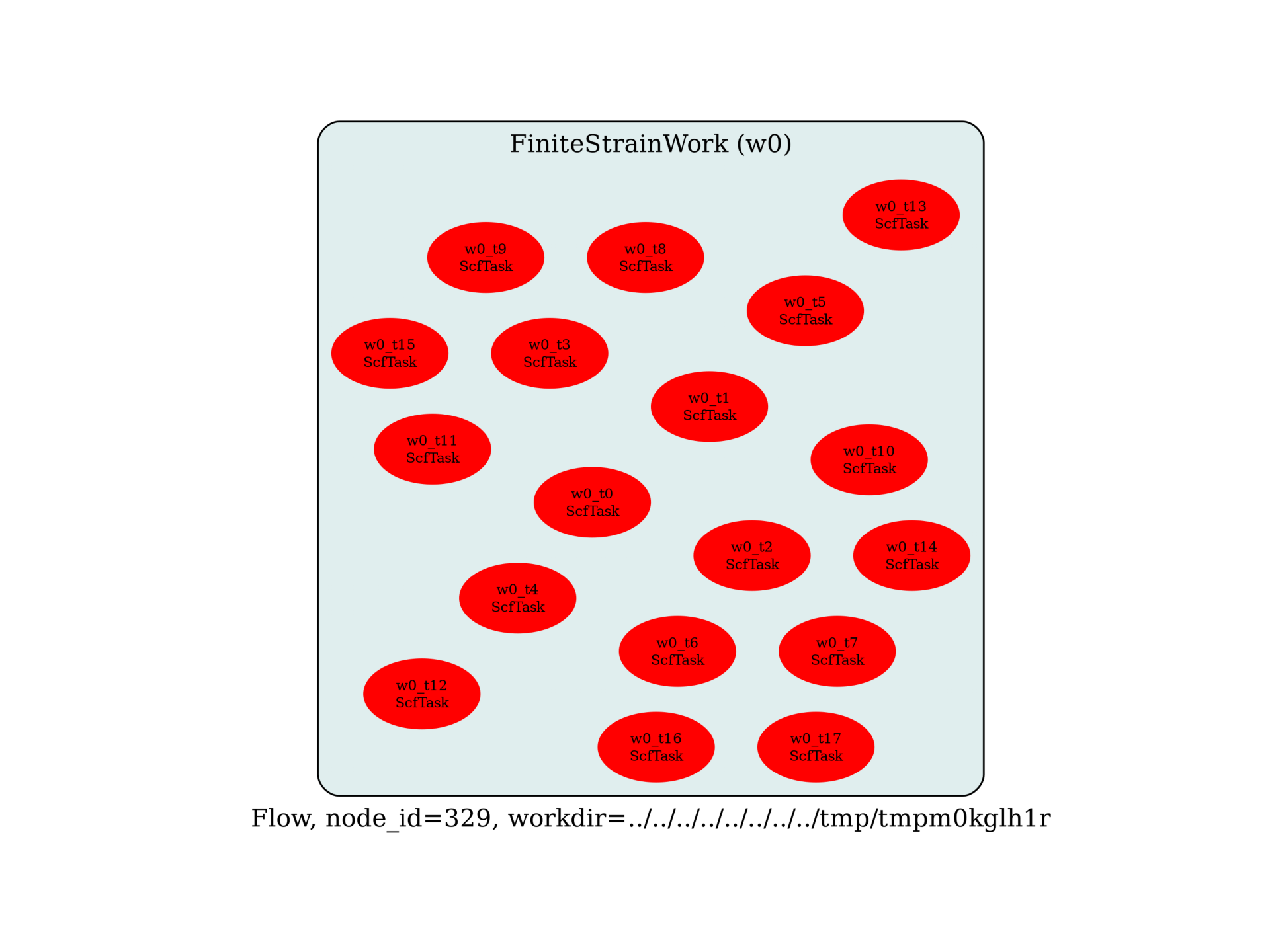
Flow to compute with finite differences.

Finite electric field calculation of AlP at clamped atomic positions

Here the polarization of the cell is computed as a function of increasing external homogeneous electric field.

berryopt 4 is used to trigger the finite field calculation, while the efield variable sets the strength (in atomic units) and direction of the field

Based on tutorespfn/Input/tpolarization_6.abi

import sys
import os
import abipy.flowtk as flowtk

from abipy.core.structure import Structure
from abipy.abio.inputs import AbinitInput
from abipy.flowtk.finitediff import FiniteStrainWork


def build_flow(options):
    # Set working directory (default is the name of the script with '.py' removed and "run_" replaced by "flow_")
    if not options.workdir:
        options.workdir = os.path.basename(sys.argv[0]).replace(".py", "").replace("run_", "flow_")

    structure = Structure.from_abistring("""
# Definition of the unit cell
acell     3*7.2728565836E+00
rprim
0.0000000000E+00  7.0710678119E-01  7.0710678119E-01
7.0710678119E-01  0.0000000000E+00  7.0710678119E-01
7.0710678119E-01  7.0710678119E-01  0.0000000000E+00

natom 2   # two atoms in the cell
typat 1 2 # type 1 is Phosphorous, type 2 is Aluminum (order defined by znucl above and pseudos list)

# Definition of the atom types and pseudopotentials
ntypat 2 # two types of atoms
znucl 15 13 # the atom types are Phosphorous and Aluminum


#atomic positions, given in units of the cell vectors. Thus as the cell vectors
#change due to strain the atoms will move as well.
xred
1/4 1/4 1/4
0 0 0
""")

    # Get NC pseudos from pseudodojo.
    from abipy.flowtk.psrepos import get_oncvpsp_pseudos
    pseudos = get_oncvpsp_pseudos(xc_name="LDA", version="0.4",
                                  relativity_type="SR", accuracy="standard")
    #nspinor = 1
    #nsppol, nspden = 1, 4
    #if nspinor == 1:
    #    nsppol, nspden  = 2, 2

    #nband 4
    # nband is restricted here to the number of filled bands only, no empty bands. The theory of
    # the Berrys phase polarization formula assumes filled bands only. Our pseudopotential choice
    # includes 5 valence electrons on P, 3 on Al, for 8 total in the primitive unit cell, hence
    # 4 filled bands.

    scf_input = AbinitInput(structure, pseudos)
    num_ele = scf_input.num_valence_electrons

    scf_input.set_vars(
        ecut=5,
        nband=4,
        tolvrs=1.0e-8,
        #toldfe=1.0e-15,
        #nspinor=nspinor,
        #nsppol=nsppol,
        #nspden=nspden,
        #nstep=7,         # Maximal number of SCF cycles from the tutorial
        nstep=50,         # Maximal number of SCF cycles
        ecutsm=0.5,
        dilatmx=1.05,
        paral_kgb=0,
    )

    shiftk = [0.5, 0.5, 0.5,
              0.5, 0.0, 0.0,
              0.0, 0.5, 0.0,
              0.0, 0.0, 0.5,
    ]
    #scf_input.set_kmesh(ngkpt=[6, 6, 6], shiftk=shiftk)
    scf_input.set_kmesh(ngkpt=[1, 1, 1], shiftk=[0, 0, 0])

    # Initialize the flow.
    flow = flowtk.Flow(workdir=options.workdir, manager=options.manager)

    fd_accuracy = 2
    relax_ions = True
    relax_ions_opts = None

    work = FiniteStrainWork.from_scf_input(
        scf_input,
        fd_accuracy=fd_accuracy,
        norm_step=0.005,
        shear_step=0.03,
        relax_ions=relax_ions,
        relax_ions_opts=relax_ions_opts,
        #extra_abivars=dict(berryopt=-1),  # This to compute the polarization at E = 0
    )

    # Add the work to the flow.
    flow.register_work(work)

    return flow


# This block generates the thumbnails in the AbiPy gallery.
# You can safely REMOVE this part if you are using this script for production runs.
if os.getenv("READTHEDOCS", False):
    __name__ = None
    import tempfile
    options = flowtk.build_flow_main_parser().parse_args(["-w", tempfile.mkdtemp()])
    build_flow(options).graphviz_imshow()


@flowtk.flow_main
def main(options):
    """
    This is our main function that will be invoked by the script.
    flow_main is a decorator implementing the command line interface.
    Command line args are stored in `options`.
    """
    return build_flow(options)


if __name__ == "__main__":
    sys.exit(main())