The ABIWAN file (wannier90)#
This notebook shows how to use AbiPy to analyze the output files
produced by wannier90 and how to use the ABIWAN.nc file
produced by Abinit to interpolate band energies.
As usual, one can use:
abiopen.py FILE_ABIWAN.nc
with the --expose or the --print option for a command line interface
and --notebook to generate a jupyter notebook.
Table of Contents#
Let’s start by importing the basic modules needed for this tutorial.
import warnings
warnings.filterwarnings("ignore")  # Ignore warnings

import os

from abipy import abilab
abilab.enable_notebook() # This line tells AbiPy we are running inside a notebook
import abipy.data as abidata

# This line configures matplotlib to show figures embedded in the notebook.
# Replace `inline` with `notebook` in classic notebook
%matplotlib inline

# Option available in jupyterlab. See https://github.com/matplotlib/jupyter-matplotlib
#%matplotlib widget
How to analyze the WOUT file#
Use abiopen to open a wout file (the main output file produced by wannier90):
filepath = os.path.join(abidata.dirpath, "refs", "wannier90", "example01_gaas.wout")

wout = abilab.abiopen(filepath)
print(wout)
================================= File Info =================================
Name: example01_gaas.wout
Directory: /home/runner/work/abipy_book/abipy_book/abipy/abipy/data/refs/wannier90
Size: 31.64 kB
Access Time: Thu Jan 15 12:16:09 2026
Modification Time: Thu Jan 15 12:15:09 2026
Change Time: Thu Jan 15 12:15:09 2026

================================= Structure =================================
Full Formula (Ga1 As1)
Reduced Formula: GaAs
abc   :   4.016499   4.016499   4.016499
angles:  60.000000  60.000000  60.000000
pbc   :       True       True       True
Sites (2)
  #  SP       a     b     c
---  ----  ----  ----  ----
  0  Ga    0     0     0
  1  As    0.25  0.25  0.25

Wannier90 version: 2.1.0+git
Number of Wannier functions: 4
K-grid: [2 2 2]

================================= WANNIERISE =================================
 iter  delta_spread  rms_gradient   spread  time     O_D     O_OD    O_TOT
    0  4.470000e+00  0.000000e+00 4.468812  0.00 0.00832 0.503629 4.468812
    1 -1.930000e-03  6.679013e-02 4.466881  0.00 0.00803 0.501988 4.466881
    2 -8.930000e-10  4.544940e-05 4.466881  0.01 0.00803 0.501988 4.466881
    3  0.000000e+00  2.000000e-10 4.466881  0.01 0.00803 0.501988 4.466881
    4  8.880000e-16  2.000000e-10 4.466881  0.01 0.00803 0.501988 4.466881
   16 -8.880000e-16  0.000000e+00 4.466881  0.02 0.00803 0.501988 4.466881
   17  8.880000e-16  0.000000e+00 4.466881  0.02 0.00803 0.501988 4.466881
   18  0.000000e+00  0.000000e+00 4.466881  0.02 0.00803 0.501988 4.466881
   19  8.880000e-16  0.000000e+00 4.466881  0.02 0.00803 0.501988 4.466881
   20  0.000000e+00  0.000000e+00 4.466881  0.02 0.00803 0.501988 4.466881
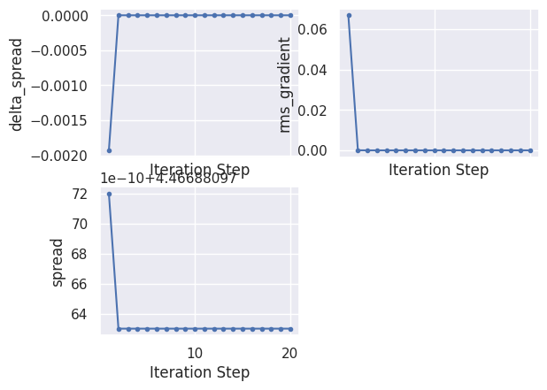
To plot the convergence of the wannier cycle use:
wout.plot();
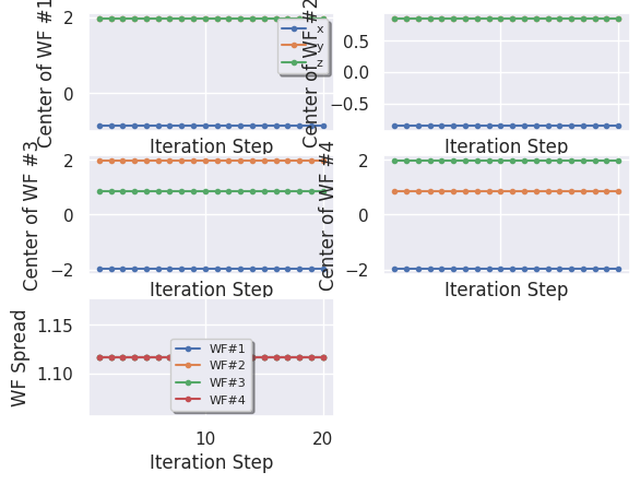
To plot the evolution of the Wannier centers and spread, use:
wout.plot_centers_spread();
Using ABIWAN.nc to interpolate band energies#
ABIWAN.nc is a netcdf file produced by Abinit after having called wannier90 in library mode.
The file contains the unitary transformation and other important parameters associated to the calculations.
This file can be read by AbiPy and can be used to interpolate band energies with the wannier method.
As usual, use abiopen to open the file:
filepath = os.path.join(abidata.dirpath, "refs", "wannier90", "tutoplugs_tw90_4", "tw90_4o_DS3_ABIWAN.nc")
abiwan = abilab.abiopen(filepath)
print(abiwan)
================================= File Info =================================
Name: tw90_4o_DS3_ABIWAN.nc
Directory: /home/runner/work/abipy_book/abipy_book/abipy/abipy/data/refs/wannier90/tutoplugs_tw90_4
Size: 205.47 kB
Access Time: Thu Jan 15 12:16:09 2026
Modification Time: Thu Jan 15 12:15:09 2026
Change Time: Thu Jan 15 12:15:09 2026

================================= Structure =================================
Full Formula (Si2)
Reduced Formula: Si
abc   :   3.840259   3.840259   3.840259
angles:  60.000000  60.000000  60.000000
pbc   :       True       True       True
Sites (2)
  #  SP       a     b     c
---  ----  ----  ----  ----
  0  Si    0     0     0
  1  Si    0.25  0.25  0.25

Abinit Spacegroup: spgid: 227, num_spatial_symmetries: 24, has_timerev: False, symmorphic: False

============================== Electronic Bands ==============================
Number of electrons: 8.0, Fermi level: 5.861 (eV)
nsppol: 1, nkpt: 64, mband: 14, nspinor: 1, nspden: 1
smearing scheme: none (occopt 1), tsmear_eV: 0.272, tsmear Kelvin: 3157.7
Direct gap:
    Energy: 2.519 (eV)
    Initial state: spin: 0, kpt: [+0.000, +0.000, +0.000], weight: 0.016, band: 3, eig: 5.861, occ: 2.000
    Final state:   spin: 0, kpt: [+0.000, +0.000, +0.000], weight: 0.016, band: 4, eig: 8.380, occ: 0.000
Fundamental gap:
    Energy: 0.635 (eV)
    Initial state: spin: 0, kpt: [+0.000, +0.000, +0.000], weight: 0.016, band: 3, eig: 5.861, occ: 2.000
    Final state:   spin: 0, kpt: [+0.500, +0.500, +0.000], weight: 0.016, band: 4, eig: 6.496, occ: 0.000
Bandwidth: 11.953 (eV)
Valence maximum located at kpt index 0:
    spin: 0, kpt: [+0.000, +0.000, +0.000], weight: 0.016, band: 3, eig: 5.861, occ: 2.000
Conduction minimum located at kpt index 10:
    spin: 0, kpt: [+0.500, +0.500, +0.000], weight: 0.016, band: 4, eig: 6.496, occ: 0.000

TIP: Use `--verbose` to print k-point coordinates with more digits
================================== K-points ==================================
K-mesh with divisions: [4, 4, 4], shifts: [0.0, 0.0, 0.0]
kptopt: 3 (Do not take into account any symmetry)
Number of points in the IBZ: 64
     0) [+0.000, +0.000, +0.000],  weight=0.016
     1) [+0.250, +0.000, +0.000],  weight=0.016
     2) [+0.500, +0.000, +0.000],  weight=0.016
     3) [-0.250, +0.000, +0.000],  weight=0.016
     4) [+0.000, +0.250, +0.000],  weight=0.016
     5) [+0.250, +0.250, +0.000],  weight=0.016
     6) [+0.500, +0.250, +0.000],  weight=0.016
     7) [-0.250, +0.250, +0.000],  weight=0.016
     8) [+0.000, +0.500, +0.000],  weight=0.016
     9) [+0.250, +0.500, +0.000],  weight=0.016
    10) [+0.500, +0.500, +0.000],  weight=0.016
    ... (More than 10 k-points)

============================= Wannier90 Results =============================
No of Wannier functions: 8, No bands: 14, Number of k-point neighbours: 8
Disentanglement: True, exclude_bands: no

WF_index  Center                     Spread
0         [1.12195 1.59353 1.59353]  2.767
1         [1.59353 1.59353 1.12195]  2.767
2         [1.12195 1.12195 1.12195]  2.767
3         [1.59353 1.12195 1.59353]  2.767
4         [0.23579 0.23579 0.23579]  2.767
5         [0.23579 2.47968 2.47968]  2.767
6         [2.47968 0.23579 2.47968]  2.767
7         [2.47968 2.47968 0.23579]  2.767
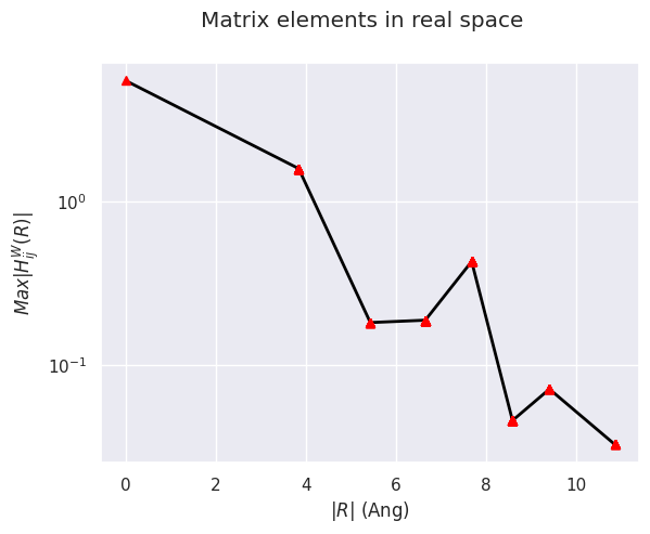
To plot the matrix elements of the KS Hamiltonian in real space in the Wannier gauge, use:
abiwan.hwan.plot(title="Matrix elements in real space");
HWanR built in 0.004 (s)
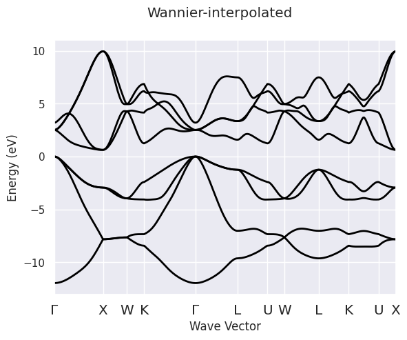
To interpolate the KS energies along a high-symmetry k-path and construct a new ElectronBands object, use:
ebands_kpath = abiwan.interpolate_ebands()
Interpolation completed in 0.016 [s]
ebands_kpath.plot(title="Wannier-interpolated");
If you need an IBZ sampling instead of a k-path, for instance a 36x36x36 k-mesh, use:
ebands_kmesh = abiwan.interpolate_ebands(ngkpt=(36, 36, 36))
Interpolation completed in 0.050 [s]
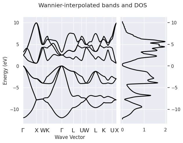
As we are dealing with AbiPy objects, we can easily reuse the AbiPy API to plot bands with DOS:
ebands_kpath.plot_with_edos(ebands_kmesh.get_edos(),
                            title="Wannier-interpolated bands and DOS");
We can also compare an ab-initio band structure with the Wannier-interpolated results. This is useful to understand if our Wannier functions are well localized, and if the k-mesh used with wannier90 is dense enough.
In this case, it is just a matter of passing the path to the netcdf file
containing the ab-initio band structure to the get_plotter_from_ebands method of abiwan.
The function interpolates the band energies using the k-path found in the netcdf file
and returns a plotter object:
import abipy.data as abidata
gsr_path = abidata.ref_file("si_nscf_GSR.nc")

plotter = abiwan.get_plotter_from_ebands(gsr_path)
---------------------------------------------------------------------------
AttributeError                            Traceback (most recent call last)
Cell In[11], line 4
      1 import abipy.data as abidata
      2 gsr_path = abidata.ref_file("si_nscf_GSR.nc")
----> 4 plotter = abiwan.get_plotter_from_ebands(gsr_path)

AttributeError: 'AbiwanFile' object has no attribute 'get_plotter_from_ebands'
Then we call combiplot to plot the two band structures on the same figure:
plotter.combiplot();
As we can see, the interpolated band structures is not completely on top of the ab-initio results. To improve the agreement we should try to reduced the spread and/or increase the density of the k-mesh used in the wannierization procedure.