
The DDB file (DFPT)#
This notebook explains how to use AbiPy and the DDB file produced by Abinit to analyze:
Phonon band structures including the LO-TO splitting in polar semiconductors
Phonon fatbands, phonon DOS and projected phonon DOS
Born effective charges \(Z^*_{\kappa,\alpha\beta}\) and the dielectric tensors \(\epsilon^{\infty}_{\alpha\beta}\), \(\epsilon^{0}_{\alpha\beta}\)
Thermodynamic properties in the harmonic approximation
In the last part, we discuss how to use the DdbRobot to analyze multiple DDB files and perform typical convergence studies.
Note
AbiPy provides two different APIs to produce figures, with either matplotlib or plotly. In this tutorial, we use the plotly API as much as possible, although it should be noted that not all the plotting methods have been ported to plotly yet.
AbiPy uses a relatively simple rule to differentiate between the two plotting libraries:
if an object provides an obj.plot method producing a matplotlib plot, the corresponding
native plotly version (if available) is named obj.plotly.
Note that plotly requires a web browser, hence the matplotlib version is still valuable if you need to
visualize results on machines on which only an X server is available.
In AbiPy versions greater than 0.9, you can try to convert the matplotlib figures produced by plot methods
into Plotly figures using the optional argument plotly=True, although the result is not always guaranteed.
Suggested references#
Integration with the Materials Project database#
AbiPy, pymatgen and fireworks have been used by Petretto et al. to compute the vibrational properties of more than 1500 compounds with Abinit. The results are available on the Materials Project website. For instance, the results for the rocksalt phase of MgO are available at https://materialsproject.org/materials/mp-1009129/.
To fetch the DDB file from the Materials Project database and build a DdbFile object, use:
ddb = abilab.DdbFile.from_mpid("mp-1009129")
Remember to set PMG_MAPI_KEY in your ~/.pmgrc.yaml as described
here.
How to create a DdbFile object#
Let us start by importing the basic AbiPy modules we have already used in the other examples:
import warnings
warnings.filterwarnings("ignore")  # Ignore warnings

from abipy import abilab
abilab.enable_notebook() # This line tells AbiPy we are running inside a notebook

import abipy.data as abidata
import os

# This line configures matplotlib to show figures embedded in the notebook.
# Replace `inline` with `notebook` in classic notebook
%matplotlib inline

# Option available in jupyterlab. See https://github.com/matplotlib/jupyter-matplotlib
#%matplotlib widget
To open a DDB file, use the high-level interface provided by abiopen:
ddb_filepath = abidata.ref_file("mp-1009129-9x9x10q_ebecs_DDB")
ddb = abilab.abiopen(ddb_filepath)
A DdbFile has a structure object:
print(ddb.structure) # Lengths in Angstrom.
Full Formula (Mg1 O1)
Reduced Formula: MgO
abc   :   2.908638   2.908638   2.656848
angles:  90.000000  90.000000 120.000000
pbc   :       True       True       True
Sites (2)
  #  SP           a         b    c
---  ----  --------  --------  ---
  0  Mg    0         0         0
  1  O     0.333333  0.666667  0.5

Abinit Spacegroup: spgid: 0, num_spatial_symmetries: 12, has_timerev: True, symmorphic: False
and a list of \(q\)-points associated with the dynamical matrix \(D(q)\):
ddb.qpoints
<abipy.core.kpoints.KpointList at 0x7f0c692aa900>
At this point, it is worth mentioning that Abinit takes advantage of symmetries to reduce the number of \(q\)-points as well as the number of perturbations that must be computed explicitly within DFPT.
The set of \(q\)-points in the DDB file does not (usually) form a homogeneous sampling of the Brillouin zone (BZ). Actually, the \(q\)-points sample the irreducible wedge (IBZ), and this sampling is obtained from an initial \(q\)-mesh specified in terms of divisions along the three reduced directions (ngqpt).
ddb.qpoints.plotly();
Note that the DDB file does not contain any information about the value of ngqpt, because an arbitrary list of \(q\)-points can be merged in the same DDB. The algorithms implemented in anaddb, however, need to know the divisions to compute integrals in the full BZ. This is indeed one of the variables that must be provided by the user in the anaddb input file.
AbiPy uses a heuristic method to guess the \(q\)-mesh from this scattered list of \(q\)-points, so that you do not need to specify this parameter when calling anaddb:
ddb.guessed_ngqpt
array([ 9, 9, 10])
Warning
If the guess is wrong, you will need to manually set this attribute to the correct value of ngqpt before
invoking anaddb from Python.
This could happen if, for instance, you have merged DDB files computed with \(q\)-points that do not belong to the same grid.
To test whether the DDB file contains the entries associated with \(\epsilon^{\infty}_{\alpha\beta}\) and \(Z^*_{\kappa,\alpha\beta}\), use:
print("Contains macroscopic dielectric tensor:", ddb.has_epsinf_terms())
print("Contains Born effective charges:", ddb.has_bec_terms())
Contains macroscopic dielectric tensor: True
Contains Born effective charges: True
Metadata are stored in the header of the DDB file. AbiPy parses this initial section and stores the values in a dict-like object. Let us print a sorted list with all the keys in the header:
from pprint import pprint
pprint(sorted(list(ddb.header.keys())))
['acell',
 'amu',
 'dfpt_sciss',
 'dilatmx',
 'ecut',
 'ecutsm',
 'intxc',
 'iscf',
 'ixc',
 'kpt',
 'kptnrm',
 'lines',
 'natom',
 'nband',
 'ngfft',
 'nkpt',
 'nspden',
 'nspinor',
 'nsppol',
 'nsym',
 'ntypat',
 'occ',
 'occopt',
 'rprim',
 'spinat',
 'symafm',
 'symrel',
 'tnons',
 'tolwfr',
 'tphysel',
 'tsmear',
 'typat',
 'usepaw',
 'version',
 'wtk',
 'xred',
 'zion',
 'znucl']
and use the standard dictionary syntax to access the values:
print("This DDB has been generated with ecut", ddb.header["ecut"], "Ha and nsym", ddb.header["nsym"])
This DDB has been generated with ecut 44.0 Ha and nsym 12
We can also print the DDB object to get a summary of the most important parameters and dimensions:
print(ddb)

# If more info is needed use:
# print(ddb.to_string(verbose=1)
================================= File Info =================================
Name: mp-1009129-9x9x10q_ebecs_DDB
Directory: /home/runner/work/abipy_book/abipy_book/abipy/abipy/data
Size: 218.73 kB
Access Time: Wed Sep 30 15:59:33 2026
Modification Time: Wed Sep 30 15:58:18 2026
Change Time: Wed Sep 30 15:58:18 2026

================================= Structure =================================
Full Formula (Mg1 O1)
Reduced Formula: MgO
abc   :   2.908638   2.908638   2.656848
angles:  90.000000  90.000000 120.000000
pbc   :       True       True       True
Sites (2)
  #  SP           a         b    c
---  ----  --------  --------  ---
  0  Mg    0         0         0
  1  O     0.333333  0.666667  0.5

Abinit Spacegroup: spgid: 0, num_spatial_symmetries: 12, has_timerev: True, symmorphic: False

================================== DDB Info ==================================

Number of q-points in DDB: 72
guessed_ngqpt: [ 9  9 10] (guess for the q-mesh divisions made by AbiPy)
ecut = 44.000000, ecutsm = 0.000000, nkpt = 405, nsym = 12, usepaw = 0
nsppol 1, nspinor 1, nspden 1, ixc = -116133, occopt = 1, tsmear = 0.010000

Has total energy: False
Has forces: False
Has stress tensor: False

Has (at least one) atomic perturbation: True
Has (at least one diagonal) electric-field perturbation: True
Has (at least one) Born effective charge: True
Has (all) strain terms: False
Has (all) internal strain terms: False
Has (all) piezoelectric terms: False
Has (all) dynamical quadrupole terms: False
If you are a terminal aficionado, remember that you can use the
abiopen.py script
to open the DDB file directly from the shell and generate a Jupyter notebook with the -nb option.
For quick visualization, use the abiview.py script.
Invoking anaddb from the DdbFile object#
The DdbFile object provides specialized methods to invoke anaddb and
compute important physical properties such as phonon band structures, phonon DOS, etc.
The names of these methods start with the ana prefix followed by a verb (anaget, anacompare).
These specialized methods:
build the anaddb input file
run anaddb
parse the netcdf files produced by anaddb
build and return AbiPy objects that can be used to plot/analyze the data.
Warning
In order to run ABINIT executables from AbiPy, you need a manager.yml with configuration options. For further details, please consult the TaskManager documentation.
The Python API is flexible and exposes several anaddb input variables. Most of the arguments have default values covering the most common scenarios, so you only need to specify them explicitly if the default behavior does not suit your needs. The most important parameters to remember are:
ndivsm: Number of divisions used for the smallest segment of the high-symmetry \(q\)-path.
nqsmall: Defines the \(q\)-mesh for the phonon DOS in terms of the number of divisions used to sample the smallest reciprocal lattice vector. Use 0 to disable the DOS computation.
lo_to_splitting: Activates the computation of the frequencies in the \(q\rightarrow 0\) limit with the inclusion of the non-analytical term (requires dipdip = 1 and a DDB with \(Z^*_{\kappa,\alpha\beta}\) and \(\epsilon^{\infty}_{\alpha\beta}\)).
The high-symmetry \(q\)-path is automatically selected assuming the structure fulfills the conventions used by Setyawan and Curtarolo, but you can also specify your own \(q\)-path if needed.
Plotting phonon bands and DOS#
To compute phonon bands and DOS, use:
# Call anaddb to compute phonon bands and DOS. Return PHBST and PHDOS netcdf files.
phbstnc, phdosnc = ddb.anaget_phbst_and_phdos_files(
    ndivsm=20, nqsmall=20, lo_to_splitting=True, asr=2, chneut=1, dipdip=1, dos_method="tetra")

# Extract phbands and phdos from the netcdf object.
phbands = phbstnc.phbands
phdos = phdosnc.phdos
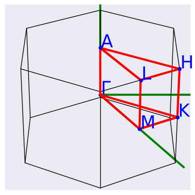
Let us have a look at the high-symmetry \(q\)-path automatically selected by AbiPy:
phbands.qpoints.plot();
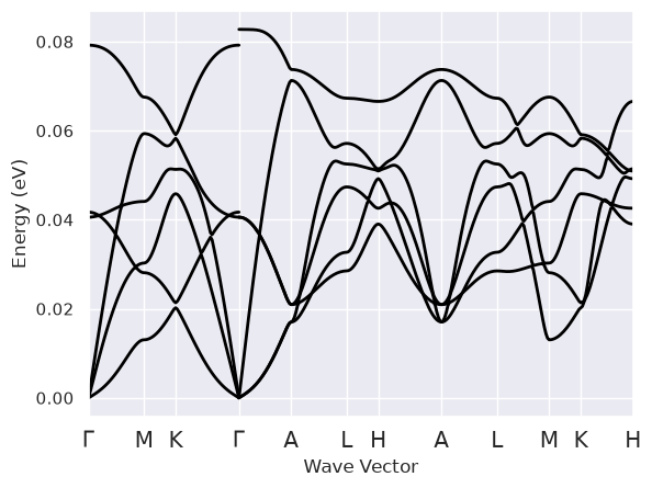
and plot the phonon bands along this path with:
phbands.plot();
phbands.plotly();
Note the discontinuity of the optical modes when we cross the \(\Gamma\) point.
In polar semiconductors, indeed, the dynamical matrix is non-analytical for \(q \rightarrow 0\).
Since lo_to_splitting was set to True, AbiPy has computed the phonon frequencies
for all the \(q \rightarrow \Gamma\) directions present in the path.
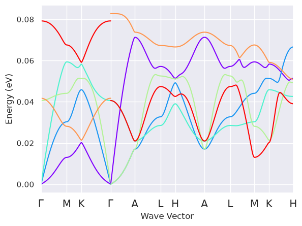
There are several band crossings and anti-crossings, hence it’s not easy to understand how the branches should be connected. Fortunately, there is a heuristic method to estimate the band connection from the overlap of the eigenvectors at adjacent \(q\)-points. To connect the modes and plot the phonon branches with different colors, use:
phbands.plot_colored_matched();
Warning
This heuristic method may fail, so the results should be analyzed critically (especially when there are non-analytic branches crossing \(\Gamma\)). Besides, the algorithm is sensitive to the resolution of the path, so it is recommended to check the results by increasing the number of points per segment.
To plot the DOS, \(g(\omega)\), and the integrated \(IDOS(\omega) = \int^{\omega}_{-\infty} g(\omega')\,d\omega'\), use:
phdos.plot();
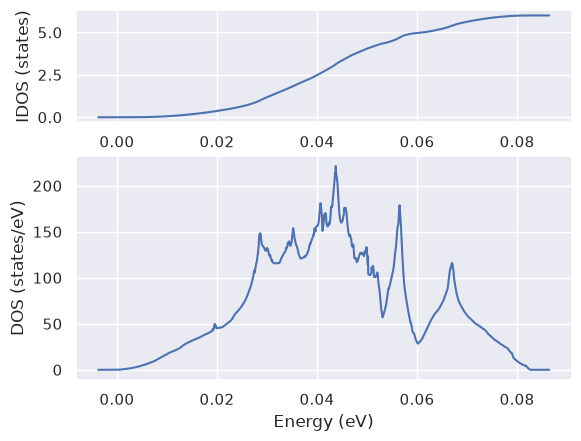
Note how the phonon DOS integrates to \(3 N_{atom} = 6\).
To plot the phonon bands and the DOS on the same figure, use:
phbands.plot_with_phdos(phdos, units="meV");
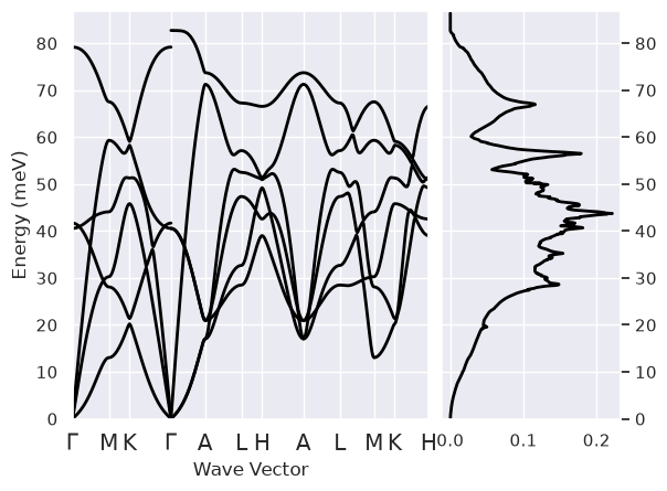
phbands.plotly_with_phdos(phdos, units="meV");
Fatbands and projected DOS#
The phbands object stores the phonon displacements, \(\vec{d}_{q\nu}\), and the eigenvectors, \(\vec{\epsilon}_{q\nu}\),
obtained by diagonalizing the dynamical matrix \(D(q)\):
We can therefore use the eigenvectors (or the displacements) to associate a width with the different bands (a.k.a. fatbands). This width gives a qualitative understanding of the vibrational modes: which atomic types are involved in the vibrations at a given energy, their direction of oscillation and their amplitude (related to the displacement).
# NB: LO-TO is not available in fatbands
phbands.plotly_fatbands(use_eigvec=True, units="Thz");
To plot the fatbands with the type-projected DOS stored in phdosnc, use:
phbands.plot_fatbands(phdos_file=phdosnc, colormap="rainbow", alpha=0.4, units="cm-1");
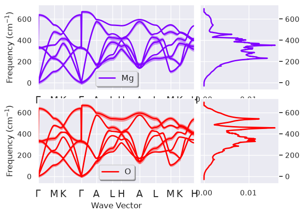
We can also plot the PJDOS summed over directions and grouped by atomic type, without fatbands:
phdosnc.plotly_pjdos_type();
The netcdf file contains the individual contributions to the total DOS for each atomic site and each of the three Cartesian directions, so there are several quantities we can plot to understand the vibrational spectrum of our system. For example, we can decide to sum over all atoms of the same type while keeping the dependence on the Cartesian direction:
phdosnc.plot_pjdos_cartdirs_type(units="Thz");
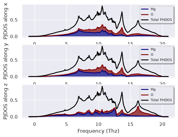
This analysis tells us that the peak at ~16 THz mainly consists of oxygen vibrations along z. We could now extend this analysis by looking at the contributions arising from the different sites with:
#phdosnc.plot_pjdos_cartdirs_site(view="inequivalent", units="eV", stacked=True);
but we prefer to stop here and discuss other tools that can be used to analyze individual phonon modes.
Visualizing atomic displacements#
If you need to visualize the lattice vibrations in 3D to gain better insight
into the nature of the phonon modes, you may want to use the phononwebsite.
You can either convert the out_PHBST.nc file produced by anaddb into JSON format
and upload it to the phononwebsite server or, alternatively, open a terminal and execute the AbiPy script:
abiview.py ddb out_DDB --phononwebsite
to automate the entire process (replace out_DDB with the name of your DDB file).
Note that other AbiPy methods are quite handy if we need to investigate the nature of the phonon modes at a particular \(q\)-point without a 3D visualization tool. For example, we can analyze the contributions of the different types of atoms to the phonon displacements at a given \(q\)-point with:
phbands.plot_phdispl(qpoint=(0, 0, 0), tight_layout=True);
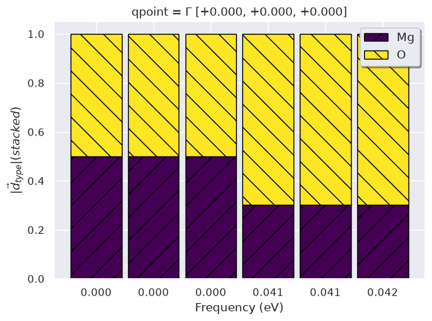
As expected, the first three (acoustic) modes have zero frequency and the two atoms oscillate with the same amplitude. These modes indeed correspond to a rigid translation of the crystal, hence the amplitude (and the direction) does not depend on the atomic site. The other three optical modes are (almost) degenerate. One would expect LO-TO splitting here, but it is absent because we are using the frequencies at the \(\Gamma\) point without the non-analytical term.
#phbands.plot_phdispl((0, 0, 0.1), is_non_analytical_direction=True, tight_layout=True);
To project the phonon displacements along the three Cartesian directions, use:
phbands.plot_phdispl_cartdirs(qpoint=(0, 0, 0.0), tight_layout=True);
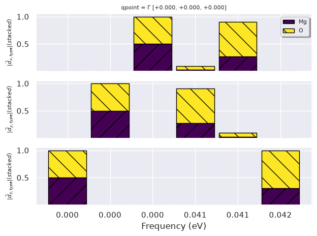
This plot confirms that the first three modes correspond to a rigid translation along x, y and z, respectively.
Analyzing the breaking of the acoustic sum rule#
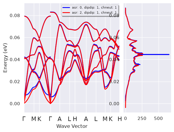
Due to the invariance of the system under an infinitesimal rigid translation, the frequencies of the lowest three modes at \(\Gamma\) should be zero. Unfortunately, all the terms that are evaluated on the real-space FFT mesh (e.g. \(V_{xc}\), non-linear core correction) break this translational invariance. The error depends on several factors (the density of the FFT mesh, pseudopotentials with hard model core charges, the XC functional, etc.). Note that it is not always possible to reduce the error to zero by just increasing the convergence parameters, but fortunately the acoustic sum rule can be restored via the asr input variable.
One can easily compare the phonon bands obtained with different values of asr with:
asr_plotter = ddb.anacompare_asr()
This method invokes anaddb with different values of asr and returns a plotter object that we can use to compare the phonon band structures:
asr_plotter.combiplot();
asr_plotter.combiplotly();
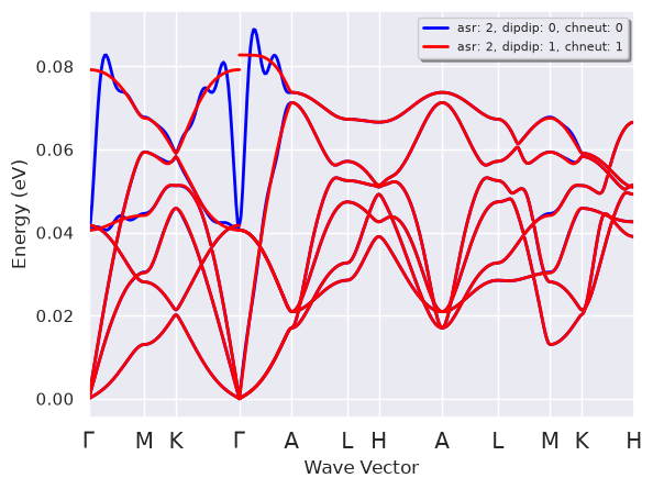
Now we can perform a similar test for the treatment of the non-analytical term in the \(q \rightarrow 0\) limit. We compute the phonon band dispersion for dipdip in [0, 1] and then compare the results on the same figure with:
dipdip_plotter = ddb.anacompare_dipdip(nqsmall=0)
dipdip_plotter.combiplot();
dipdip_plotter.combiplotly();
The figure above shows that the (Fourier-interpolated) bands obtained with dipdip = 0 have unphysical oscillations around the \(\Gamma\) point. These oscillations are due to the long-range behavior in real space of the interatomic force constants in polar semiconductors. Describing this long-range term correctly without dipdip = 1 would require an extremely dense \(q\)-point mesh in the DFPT calculation.
With dipdip = 1, on the other hand, we can model this long-range behavior in terms of a dipole-dipole interaction involving the Born effective charges and the macroscopic dielectric tensor. This allows us to decompose the full dynamical matrix into:
The analytical part of the dynamical matrix, \(D^{sr}(q)\), is short-ranged and can be Fourier-interpolated with a relatively coarse \(q\)-mesh. Then the model for the non-analytical term, \(D^{dip-dip}(q)\), is added back to the interpolated matrix to get the full dynamical matrix. This procedure removes the unphysical oscillations and is required to correctly describe the non-analytical behavior of the optical modes for \(q \rightarrow 0\).
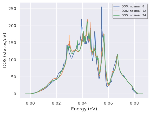
Computing DOS with different q-meshes#
The phonon DOS and derived quantities (e.g. thermodynamic properties) are sensitive to the BZ sampling, and dense meshes may be required to converge the final results.
The anacompare_phdos method provides a simple interface to
compare phonon DOS computed with different \(q\)-meshes.
We only need to provide a list of integers (nqsmalls). Each integer defines the number of divisions used to
sample the smallest reciprocal lattice vector, while the other two vectors are sampled such
that proportions are preserved.
To compute three phonon DOS with an increasing number of \(q\)-points, use:
res = ddb.anacompare_phdos(nqsmalls=[8, 12, 24])
The return value is a named tuple: res.phdoses contains the phonon DOSes, while res.plotter
is a PhononDosPlotter.
We can easily compare our results with:
res.plotter.combiplot();
Thermodynamic properties in the harmonic approximation#
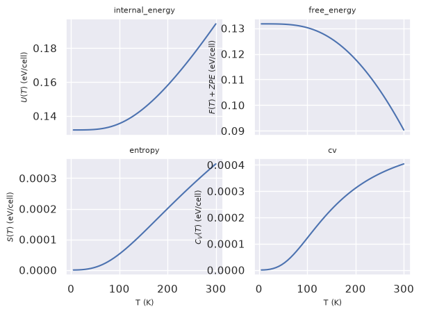
The thermodynamic properties of an ensemble of non-interacting phonons can be expressed in terms of integrals of the phonon DOS \(g(\omega)\) using:
where \(k_B\) is the Boltzmann constant. This is a reasonable approximation, especially in the low-temperature regime, where anharmonic effects can be neglected.
Let’s plot the vibrational contributions to the thermodynamic properties as a function of the temperature \(T\):
phdos.plot_harmonic_thermo();
and the zero-point energy \(\dfrac{1}{2 N_q} \sum_{q\nu} \omega_{q\nu}\):
zpe = phdos.zero_point_energy
print("Zero-point energy", zpe, zpe.to("Ha"))
Zero-point energy 0.13171156295558706 eV 0.004840310661315252 Ha
To get the free energy for a range of temperatures (in Kelvin), use:
f = phdos.get_free_energy(tstart=10, tstop=100)
#f.plot();
Macroscopic dielectric tensor and Born effective charges#
Let us call anaddb to compute the electronic contribution to the macroscopic dielectric tensor, \(\epsilon^{\infty}_{\alpha\beta}\), and the Born effective charges \(Z^*_{\kappa,\alpha\beta}\):
emacro, becs = ddb.anaget_epsinf_and_becs(chneut=1)
Note the use of chneut to enforce charge neutrality.
emacro
| x | y | z | |
|---|---|---|---|
| x | 3.438497 | 0.000000 | 0.000000 |
| y | 0.000000 | 3.438497 | 0.000000 |
| z | 0.000000 | 0.000000 | 3.499416 |
becs
| element | site_index | frac_coords | wyckoff | xx | yy | zz | xy | xz | yx | yz | zx | zy | |
|---|---|---|---|---|---|---|---|---|---|---|---|---|---|
| 0 | Mg | 0 | [0.0, 0.0, 0.0] | 1a | 1.98721 | 1.98721 | 2.10659 | 0.0 | 2.565407e-24 | 0.0 | 1.629252e-23 | 0.0 | 0.0 |
| 1 | O | 1 | [0.33333333333333, 0.66666666666667, 0.5] | 1d | -1.98721 | -1.98721 | -2.10659 | 0.0 | -2.565407e-24 | 0.0 | -1.629252e-23 | 0.0 | 0.0 |
To compute the low-frequency (infrared) dielectric tensor, \(\epsilon^{0}_{\alpha\beta}\), one has to include the response of the ions, whose motion is triggered by the electric field. One can show that:
where \(\omega^{\Gamma}_m\) are the phonon frequencies at the center of the BZ and \(S_{m,\alpha\beta}\) is the so-called mode-oscillator strength tensor, which depends on the phonon displacements and the Born effective charges.
To compute the dielectric tensor using the data stored in the DDB file, use:
dtgen = ddb.anaget_dielectric_tensor_generator()
# call print to get useful information
print(dtgen)
================================= Structure =================================
Full Formula (Mg1 O1)
Reduced Formula: MgO
abc   :   2.908638   2.908638   2.656848
angles:  90.000000  90.000000 120.000000
pbc   :       True       True       True
Sites (2)
  #  SP           a         b    c
---  ----  --------  --------  ---
  0  Mg    0         0         0
  1  O     0.333333  0.666667  0.5

Abinit Spacegroup: spgid: 1, num_spatial_symmetries: 12, has_timerev: True, symmorphic: False

============================ Oscillator strength ============================
Real part in Cartesian coordinates. a.u. units; 1 a.u. = 253.2638413 m3/s2. Set to zero below 1.00e-06.
                          xx                      yy                     zz   yz   xz   xy
mode
0                        0.0                     0.0                    0.0  0.0  0.0  0.0
1                        0.0                     0.0                    0.0  0.0  0.0  0.0
2                        0.0                     0.0                    0.0  0.0  0.0  0.0
3     0.00022453328281351966                     0.0                    0.0  0.0  0.0  0.0
4                        0.0  0.00022453328281351966                    0.0  0.0  0.0  0.0
5                        0.0                     0.0  0.0002523207013218457  0.0  0.0  0.0

============================= Dielectric Tensors =============================
Electronic dielectric tensor (eps_inf) in Cartesian coordinates. Set to zero below 1.00e-03.
          x         y         z
x  3.438497  0.000000  0.000000
y  0.000000  3.438497  0.000000
z  0.000000  0.000000  3.499416

Zero-frequency dielectric tensor (eps_zero) in Cartesian coordinates. Set to zero below 1.00e-03.
           x          y          z
x  13.101919   0.000000   0.000000
y   0.000000  13.101919   0.000000
z   0.000000   0.000000  13.779005
To compute the tensor for a given frequency:
e0 = dtgen.tensor_at_frequency(0)
print(e0)
[[ 1.31018620e+01+0.02381961j  2.54893071e-16+0.j
   1.47502725e-25+0.j        ]
 [ 0.00000000e+00+0.j          1.31018620e+01+0.02381961j
  -2.55482215e-25+0.j        ]
 [-3.68756813e-25+0.j         -1.27741107e-25+0.j
   1.37789478e+01+0.02465278j]]
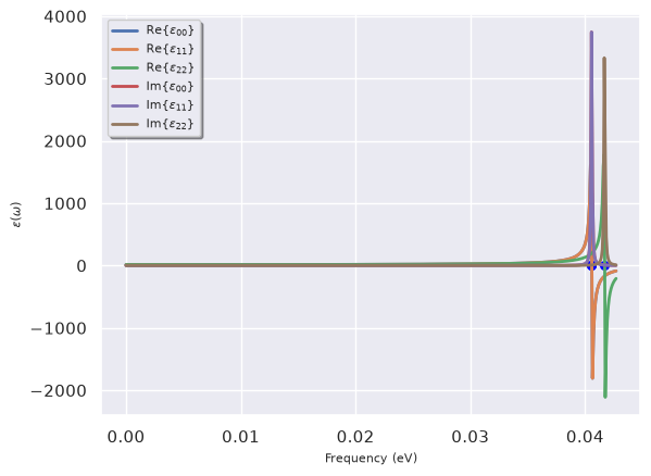
To plot the frequency dependence with a damping factor of 1e-4 eV (phonon linewidth):
dtgen.plot(w_max=None, gamma_ev=1e-4, component='diag', units='eV');
Using DdbRobot to perform convergence studies#
A DdbRobot receives a list of DDB files and provides methods
to construct pandas dataframes
and analyze the results of multiple calculations.
In particular, DdbRobots are extremely useful to study the convergence of the phonon frequencies with respect to computational parameters such as the number of \(k\)-points and the electronic smearing in metallic systems.
In this example, we are interested in the effect of the \(k\)-point sampling and of the smearing parameter
on the vibrational properties of magnesium diboride.
MgB\(_2\) is a metallic system with a critical temperature of 39 K, the highest among conventional
(phonon-mediated) superconductors.
We use precomputed DDB files obtained by running GS+DFPT calculations with different values
of nkpt and tsmear.
Let’s build our DdbRobot object with:
import os
paths = [
    #"mgb2_444k_0.01tsmear_DDB",
    #"mgb2_444k_0.02tsmear_DDB",
    #"mgb2_444k_0.04tsmear_DDB",
    "mgb2_888k_0.01tsmear_DDB",
    "mgb2_888k_0.02tsmear_DDB",
    "mgb2_888k_0.04tsmear_DDB",
    "mgb2_121212k_0.01tsmear_DDB",
    "mgb2_121212k_0.02tsmear_DDB",
    "mgb2_121212k_0.04tsmear_DDB",
]

paths = [os.path.join(abidata.dirpath, "refs", "mgb2_phonons_nkpt_tsmear", f) for f in paths]

robot = abilab.DdbRobot.from_files(paths)
robot
- ../abipy/abipy/data/refs/mgb2_phonons_nkpt_tsmear/mgb2_888k_0.01tsmear_DDB
- ../abipy/abipy/data/refs/mgb2_phonons_nkpt_tsmear/mgb2_888k_0.02tsmear_DDB
- ../abipy/abipy/data/refs/mgb2_phonons_nkpt_tsmear/mgb2_888k_0.04tsmear_DDB
- ../abipy/abipy/data/refs/mgb2_phonons_nkpt_tsmear/mgb2_121212k_0.01tsmear_DDB
- ../abipy/abipy/data/refs/mgb2_phonons_nkpt_tsmear/mgb2_121212k_0.02tsmear_DDB
- ../abipy/abipy/data/refs/mgb2_phonons_nkpt_tsmear/mgb2_121212k_0.04tsmear_DDB
The abicomp.py script provides a command-line interface to build robots from a list of files/directories given as arguments.
The DDB files are now stored in the robot with a label constructed from the file path. These labels, however, are not very informative. Ideally, we would like labels that reflect the values of (nkpt, tsmear), also because these labels will be used in our plots.
Let’s fix this with a function that recomputes the labels from the metadata available in ddb.header:
function = lambda ddb: "nkpt: %s, tsmear: %.2f" % (ddb.header["nkpt"], ddb.header["tsmear"])
robot.remap_labels(function);
robot
- nkpt: 256, tsmear: 0.01
- nkpt: 256, tsmear: 0.02
- nkpt: 256, tsmear: 0.04
- nkpt: 864, tsmear: 0.01
- nkpt: 864, tsmear: 0.02
- nkpt: 864, tsmear: 0.04
We are usually interested in the convergence behavior with respect to one or two parameters of the calculation. Let’s build a pandas dataframe with the most important parameters extracted from the DDB headers:
robot.get_params_dataframe()
| nkpt | nsppol | ecut | tsmear | occopt | ixc | nband | usepaw | |
|---|---|---|---|---|---|---|---|---|
| nkpt: 256, tsmear: 0.01 | 256 | 1 | 35.0 | 0.01 | 4 | 1 | 8 | 0 |
| nkpt: 256, tsmear: 0.02 | 256 | 1 | 35.0 | 0.02 | 4 | 1 | 8 | 0 |
| nkpt: 256, tsmear: 0.04 | 256 | 1 | 35.0 | 0.04 | 4 | 1 | 8 | 0 |
| nkpt: 864, tsmear: 0.01 | 864 | 1 | 35.0 | 0.01 | 4 | 1 | 8 | 0 |
| nkpt: 864, tsmear: 0.02 | 864 | 1 | 35.0 | 0.02 | 4 | 1 | 8 | 0 |
| nkpt: 864, tsmear: 0.04 | 864 | 1 | 35.0 | 0.04 | 4 | 1 | 8 | 0 |
Now we tell the robot to invoke anaddb to compute the phonon bands for all the DDB files.
Since we are not interested in the phonon DOS, nqsmall is set to 0:
r = robot.anaget_phonon_plotters(nqsmall=0)
Now we can plot all the phonon band structures on the same figure with:
r.phbands_plotter.combiplot();
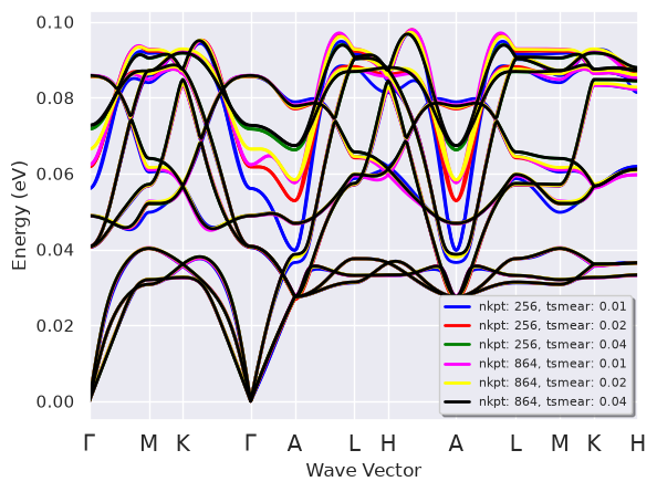
The plot is a bit crowded. Still, it is clear that some portions of the vibrational spectrum are quite sensitive to the values of (nkpt, tsmear).
In metals, it’s common to analyze the convergence of physical properties by plotting the results as a function of the \(k\)-point sampling for a fixed value of tsmear. Let’s do something similar for the phonon band structures:
r.phbands_plotter.gridplot_with_hue("tsmear", units="Thz");
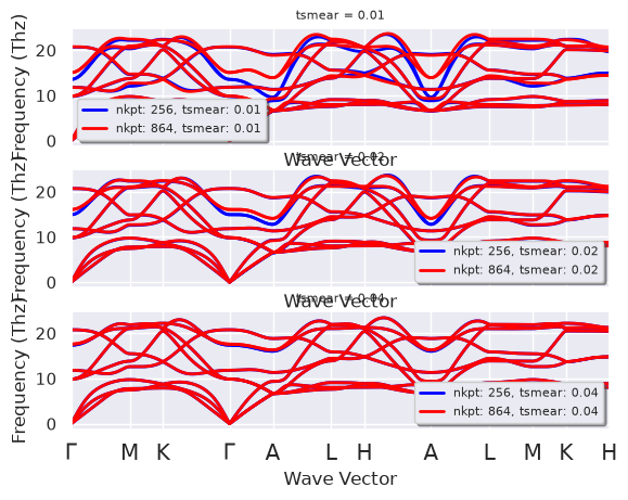
Each panel now shows the phonon dispersion computed with different \(k\)-point samplings at fixed tsmear.
The results obtained with the largest broadening (0.04 Ha) seem to be converged, but remember that “converged” results are, in principle, obtained in the limit \(nkpt \rightarrow +\infty\) and \(tsmear\rightarrow 0\). In practice, it is not always possible to reach the mathematical limit, so we should try to understand what happens to our observables when we approach this limit, and whether we can find values of (nkpt, tsmear) that are “close enough” to convergence.
The middle panel reveals that two branches (6-7, Python indexing) along \(\Gamma-A\) are quite sensitive to the sampling of the Fermi surface, and this picture is confirmed by the first panel, obtained with the lowest value of the electronic broadening.
This analysis tells us two things:
We should analyze in more detail the convergence behavior of these specific branches with respect to (nkpt, tsmear) to make sure our results are really converged.
The strong variations observed in that particular region of the phonon spectrum could be the signature of a strong coupling between these vibrational modes and the electrons on the Fermi surface.
If you dig a bit into the scientific literature, you will find that this is the famous \(E_{2g}\) branch (in-plane oscillations of the two B atoms, twofold degenerate at \(\Gamma\)), which plays an important role in explaining the superconducting behavior of MgB\(_2\).
Let’s look in more detail at the softening at the \(\Gamma\) point.
We start by calling get_phdata_at_qpoint to construct a pandas dataframe
with the phonon frequencies in meV and the parameters of the calculation:
data = robot.get_phdata_at_qpoint(qpoint=(0, 0, 0), with_geo=False)
Calculation completed. Anaddb results available in: /tmp/tmpyrthfvek
Calculation completed. Anaddb results available in: /tmp/tmp28h3ns7z
Calculation completed. Anaddb results available in: /tmp/tmp0rrgpavi
Calculation completed. Anaddb results available in: /tmp/tmp3ra3le4_
Calculation completed. Anaddb results available in: /tmp/tmpbv00z6se
Calculation completed. Anaddb results available in: /tmp/tmp__fv1c6g
and use seaborn to produce a scatter plot in which the color of the points depends on tsmear:
robot.plot_xy_with_hue(data.ph_df, x="nkpt", y="mode6", hue="tsmear");
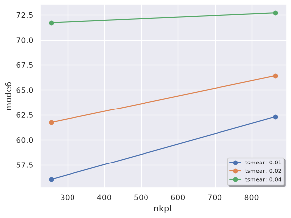
A DdbRobot is essentially a dictionary of DdbFile objects, so we can reuse the DdbFile methods to call anaddb.
For example, we mentioned that the two degenerate \(E_{2g}\) modes at \(\Gamma\) involve in-plane oscillations of the two B atoms.
Let’s check this with:
key = "nkpt: 864, tsmear: 0.04"
gamma_point = (0, 0, 0)

phbands_gamma = robot[key].anaget_phmodes_at_qpoint(gamma_point, dipdip=0, lo_to_splitting=False)
phbands_gamma.plot_phdispl_cartdirs(gamma_point);
Calculation completed. Anaddb results available in: /tmp/tmpa1zjsz8u
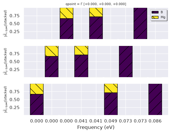
How to analyze the convergence of \(\epsilon^0\), \(\epsilon^\infty\) and Born effective charges#
Let’s assume we have computed the dielectric properties and the Born effective charges of a given
system with different \(k\)-meshes, and we want to analyze the convergence of the results.
Also in this case, the DdbRobot provides methods to automate most of the boring work.
As usual, we start by creating a robot from a list of paths to DDB files. Here we use four files produced with 2x2x2, 4x4x4, 6x6x6 and 8x8x8 \(k\)-meshes.
paths = [
"AlAs_222k_DDB",
"AlAs_444k_DDB",
"AlAs_666k_DDB",
"AlAs_888k_DDB",
]

paths = [os.path.join(abidata.dirpath, "refs", "alas_eps_and_becs_vs_ngkpt", f) for f in paths]

alas_robot = abilab.DdbRobot.from_files(paths)
Now we call anacompare_epsinf to create a pandas DataFrame with the upper triangle
of the \(\epsilon_{ij}^\infty\) dielectric tensor (Voigt notation), and we add the number of \(k\)-points
in the IBZ to the table to facilitate the analysis:
epsinf_data = alas_robot.anacompare_epsinf(ddb_header_keys="nkpt")
epsinf_data.df
| xx | yy | zz | yz | xz | xy | formula | chneut | nkpt | |
|---|---|---|---|---|---|---|---|---|---|
| 0 | 12.996449 | 12.996449 | 12.996449 | 0.0 | 0.0 | 0.0 | Al1 As1 | 1 | 16 |
| 1 | 9.268431 | 9.268431 | 9.268431 | 0.0 | 0.0 | 0.0 | Al1 As1 | 1 | 128 |
| 2 | 8.881665 | 8.881665 | 8.881665 | 0.0 | 0.0 | 0.0 | Al1 As1 | 1 | 432 |
| 3 | 8.818122 | 8.818122 | 8.818122 | 0.0 | 0.0 | 0.0 | Al1 As1 | 1 | 1024 |
epsinf_data.plot_conv("nkpt", abs_conv=0.1)
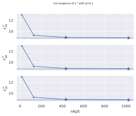
A similar approach can be used to analyze \(\epsilon_{ij}^0\):
r = alas_robot.anacompare_eps0(ddb_header_keys="nkpt")
r.df
| xx | yy | zz | yz | xz | xy | formula | asr | chneut | nkpt | |
|---|---|---|---|---|---|---|---|---|---|---|
| 0 | 15.205414 | 15.205414 | 15.205414 | 0.0 | 0.0 | 0.0 | Al1 As1 | 2 | 1 | 16 |
| 1 | 10.839420 | 10.839420 | 10.839420 | 0.0 | 0.0 | 0.0 | Al1 As1 | 2 | 1 | 128 |
| 2 | 10.423517 | 10.423517 | 10.423517 | 0.0 | 0.0 | 0.0 | Al1 As1 | 2 | 1 | 432 |
| 3 | 10.352747 | 10.352747 | 10.352747 | 0.0 | 0.0 | 0.0 | Al1 As1 | 2 | 1 | 1024 |
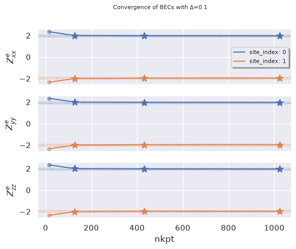
Analyzing the convergence of the Born effective charges is a bit more complicated because now we have a tensor for each atom in the unit cell:
becs_data = alas_robot.anacompare_becs(ddb_header_keys="nkpt")
becs_data.df
| element | site_index | frac_coords | wyckoff | xx | yy | zz | xy | xz | yx | yz | zx | zy | formula | chneut | nkpt | |
|---|---|---|---|---|---|---|---|---|---|---|---|---|---|---|---|---|
| 0 | Al | 0 | [0.0, 0.0, 0.0] | 1a | 2.344626 | 2.344626 | 2.344626 | 0.0 | 3.443860e-19 | 0.0 | 3.443860e-19 | 0.0 | 0.0 | Al1 As1 | 1 | 16 |
| 2 | Al | 0 | [0.0, 0.0, 0.0] | 1a | 1.998460 | 1.998460 | 1.998460 | 0.0 | 4.579838e-20 | 0.0 | 4.579838e-20 | 0.0 | 0.0 | Al1 As1 | 1 | 128 |
| 6 | Al | 0 | [0.0, 0.0, 0.0] | 1a | 1.967000 | 1.967000 | 1.967000 | 0.0 | 1.580002e-20 | 0.0 | 1.580002e-20 | 0.0 | 0.0 | Al1 As1 | 1 | 1024 |
| 4 | Al | 0 | [0.0, 0.0, 0.0] | 1a | 1.972550 | 1.972550 | 1.972550 | 0.0 | 1.519421e-19 | 0.0 | 1.519421e-19 | 0.0 | 0.0 | Al1 As1 | 1 | 432 |
| 3 | As | 1 | [0.25, 0.25, 0.25] | 1d | -1.998460 | -1.998460 | -1.998460 | 0.0 | -4.579838e-20 | 0.0 | -4.579838e-20 | 0.0 | 0.0 | Al1 As1 | 1 | 128 |
| 1 | As | 1 | [0.25, 0.25, 0.25] | 1d | -2.344626 | -2.344626 | -2.344626 | 0.0 | -3.443860e-19 | 0.0 | -3.443860e-19 | 0.0 | 0.0 | Al1 As1 | 1 | 16 |
| 5 | As | 1 | [0.25, 0.25, 0.25] | 1d | -1.972550 | -1.972550 | -1.972550 | 0.0 | -1.519421e-19 | 0.0 | -1.519421e-19 | 0.0 | 0.0 | Al1 As1 | 1 | 432 |
| 7 | As | 1 | [0.25, 0.25, 0.25] | 1d | -1.967000 | -1.967000 | -1.967000 | 0.0 | -1.580002e-20 | 0.0 | -1.580002e-20 | 0.0 | 0.0 | Al1 As1 | 1 | 1024 |
becs_data.plot_conv("nkpt", abs_conv=0.1);
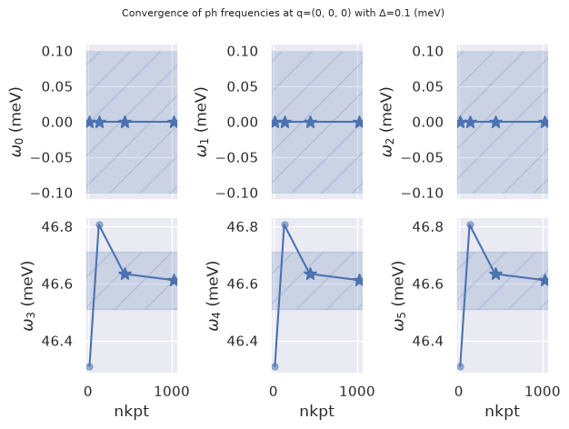
A similar API can be used to analyze the convergence of the phonon frequencies at a given \(q\)-point:
ph_data = alas_robot.get_phdata_at_qpoint(qpoint=(0, 0, 0))
ph_data.ph_df
Calculation completed. Anaddb results available in: /tmp/tmpwxgqxuld
Calculation completed. Anaddb results available in: /tmp/tmpnb1mul0k
Calculation completed. Anaddb results available in: /tmp/tmprn89yc6i
Calculation completed. Anaddb results available in: /tmp/tmpbqudp68f
| mode0 | mode1 | mode2 | mode3 | mode4 | mode5 | nkpt | nsppol | ecut | tsmear | ... | beta | gamma | a | b | c | volume | abispg_num | spglib_symb | spglib_num | spglib_lattice_type | |
|---|---|---|---|---|---|---|---|---|---|---|---|---|---|---|---|---|---|---|---|---|---|
| ../abipy/abipy/data/refs/alas_eps_and_becs_vs_ngkpt/AlAs_222k_DDB | 0.0 | 0.0 | 0.0 | 46.309323 | 46.309323 | 46.309323 | 16 | 1 | 2.0 | 0.01 | ... | 60.0 | 60.0 | 3.970101 | 3.970101 | 3.970101 | 44.247584 | 1 | F-43m | 216 | cubic |
| ../abipy/abipy/data/refs/alas_eps_and_becs_vs_ngkpt/AlAs_444k_DDB | 0.0 | 0.0 | 0.0 | 46.805652 | 46.805652 | 46.805652 | 128 | 1 | 2.0 | 0.01 | ... | 60.0 | 60.0 | 3.970101 | 3.970101 | 3.970101 | 44.247584 | 1 | F-43m | 216 | cubic |
| ../abipy/abipy/data/refs/alas_eps_and_becs_vs_ngkpt/AlAs_666k_DDB | 0.0 | 0.0 | 0.0 | 46.633272 | 46.633272 | 46.633272 | 432 | 1 | 2.0 | 0.01 | ... | 60.0 | 60.0 | 3.970101 | 3.970101 | 3.970101 | 44.247584 | 1 | F-43m | 216 | cubic |
| ../abipy/abipy/data/refs/alas_eps_and_becs_vs_ngkpt/AlAs_888k_DDB | 0.0 | 0.0 | 0.0 | 46.611452 | 46.611452 | 46.611452 | 1024 | 1 | 2.0 | 0.01 | ... | 60.0 | 60.0 | 3.970101 | 3.970101 | 3.970101 | 44.247584 | 1 | F-43m | 216 | cubic |
4 rows × 27 columns
ph_data.plot_ph_conv("nkpt", abs_conv=0.1); # meV units.
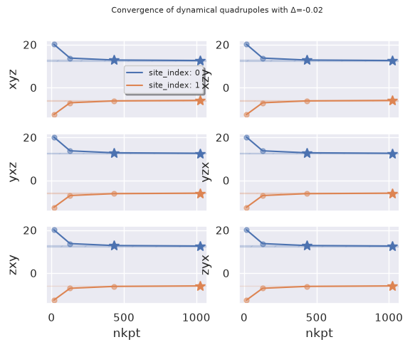
If the DDB contains dynamical quadrupoles, a similar dataframe with the tensor
elements is automatically built and made available in ph_data.dyn_quad_df.
ph_data.dyn_quad_df
| element | site_index | frac_coords | wyckoff | xxx | xxy | xxz | xyx | xyy | xyz | ... | spglib_num | spglib_lattice_type | nkpt | nsppol | ecut | tsmear | occopt | ixc | nband | usepaw | |
|---|---|---|---|---|---|---|---|---|---|---|---|---|---|---|---|---|---|---|---|---|---|
| 0 | Al | 0 | [0.0, 0.0, 0.0] | 1a | -2.243078e-08 | -2.415429e-09 | -2.415429e-09 | -2.415429e-09 | 0.0 | 20.138754 | ... | 216 | cubic | 16 | 1 | 2.0 | 0.01 | 1 | 1 | 4 | 0 |
| 1 | As | 1 | [0.25, 0.25, 0.25] | 1d | -1.088089e-07 | -3.286597e-09 | -3.286597e-09 | -3.286597e-09 | 0.0 | -12.586486 | ... | 216 | cubic | 16 | 1 | 2.0 | 0.01 | 1 | 1 | 4 | 0 |
| 2 | Al | 0 | [0.0, 0.0, 0.0] | 1a | -3.570443e-08 | -2.209766e-08 | -2.209766e-08 | -2.209766e-08 | 0.0 | 13.726256 | ... | 216 | cubic | 128 | 1 | 2.0 | 0.01 | 1 | 1 | 4 | 0 |
| 3 | As | 1 | [0.25, 0.25, 0.25] | 1d | -9.438199e-08 | -4.579025e-08 | -4.579025e-08 | -4.579025e-08 | 0.0 | -7.083927 | ... | 216 | cubic | 128 | 1 | 2.0 | 0.01 | 1 | 1 | 4 | 0 |
| 4 | Al | 0 | [0.0, 0.0, 0.0] | 1a | -3.065937e-08 | -1.837058e-08 | -1.837058e-08 | -1.837058e-08 | 0.0 | 12.813336 | ... | 216 | cubic | 432 | 1 | 2.0 | 0.01 | 1 | 1 | 4 | 0 |
| 5 | As | 1 | [0.25, 0.25, 0.25] | 1d | -1.021827e-07 | -4.617914e-08 | -4.617914e-08 | -4.617914e-08 | 0.0 | -6.205913 | ... | 216 | cubic | 432 | 1 | 2.0 | 0.01 | 1 | 1 | 4 | 0 |
| 6 | Al | 0 | [0.0, 0.0, 0.0] | 1a | -2.744198e-08 | -1.517858e-08 | -1.517858e-08 | -1.517858e-08 | 0.0 | 12.588533 | ... | 216 | cubic | 1024 | 1 | 2.0 | 0.01 | 1 | 1 | 4 | 0 |
| 7 | As | 1 | [0.25, 0.25, 0.25] | 1d | -9.765058e-08 | -4.402063e-08 | -4.402063e-08 | -4.402063e-08 | 0.0 | -5.989993 | ... | 216 | cubic | 1024 | 1 | 2.0 | 0.01 | 1 | 1 | 4 | 0 |
8 rows × 52 columns
A negative value of abs_conv is interpreted as a relative convergence criterion:
ph_data.plot_dyn_quad_conv("nkpt", abs_conv=-0.02);