The FATBANDS.nc file#
The FATBANDS.nc file contains the projection of the KS wavefunctions onto atom-centered functions with given angular momentum \(l\).
The file is generated by using the prtdos variable either in a SCF or NSCF run.
One can use the abiopen function provided by abilab to open the file and generate an instance of FatbandsFile.
Alternatively, use the abiopen.py script to open the file inside the shell with the syntax:
abiopen.py out_FATBANDS.nc
This command will start the ipython interpreter so that one can interact directly
with the FatbandFile object (named obj inside ipython).
To generate a jupyter notebook use:
abiopen.py out_FATBANDS.nc -nb
For a quick visualization of the data, use:
abiopen.py out_FATBANDS.nc -e
Note
AbiPy provides two different APIs to produce figures either with matplotlib or with plotly. In this tutorial, we will use the plotly API as much as possible although it should be noted that not all the plotting methods have been yet ported to plotly.
AbiPy uses a relatively simple rule to differentiate between the two plotting libraries:
if an object provides an obj.plot method producing a matplotlib plot, the corresponding
native plotly version (if available) is named obj.plotly.
Note that plotly requires a web browser hence the matplotlib version is still valuable if you need to
visualize results on machines in which only the X-server is available.
In AbiPy versions greater than 0.9, it is possible to try converting matplotlib figures produce by plot methods
into Plotly figures using the optional argument plotly=True, although the result is not always guaranteed.
import warnings
warnings.filterwarnings("ignore")  # Ignore warnings

from abipy import abilab
abilab.enable_notebook() # This line tells AbiPy we are running inside a notebook
import abipy.data as abidata

# This line configures matplotlib to show figures embedded in the notebook.
# Replace `inline` with `notebook` in classic notebook
%matplotlib inline

# Option available in jupyterlab. See https://github.com/matplotlib/jupyter-matplotlib
#%matplotlib widget
# This fatbands file has been produced on a k-path so it is not suitable for DOS calculations.
fbnc_kpath = abilab.abiopen(abidata.ref_file("mgb2_kpath_FATBANDS.nc"))
To print file info i.e., dimensions, variables, etc. (note that prtdos = 3, so LM decomposition is not available)
print(fbnc_kpath)
================================= File Info =================================
Name: mgb2_kpath_FATBANDS.nc
Directory: /home/runner/work/abipy_book/abipy_book/abipy/abipy/data/refs/mgb2_fatbands
Size: 149.01 kB
Access Time: Thu Jan 15 12:18:23 2026
Modification Time: Thu Jan 15 12:15:09 2026
Change Time: Thu Jan 15 12:15:09 2026

================================= Structure =================================
Full Formula (Mg1 B2)
Reduced Formula: MgB2
abc   :   3.086000   3.086000   3.523000
angles:  90.000000  90.000000 120.000000
pbc   :       True       True       True
Sites (3)
  #  SP           a         b    c
---  ----  --------  --------  ---
  0  Mg    0         0         0
  1  B     0.333333  0.666667  0.5
  2  B     0.666667  0.333333  0.5

Abinit Spacegroup: spgid: 191, num_spatial_symmetries: 24, has_timerev: True, symmorphic: False

============================== Electronic Bands ==============================
================================= Structure =================================
Full Formula (Mg1 B2)
Reduced Formula: MgB2
abc   :   3.086000   3.086000   3.523000
angles:  90.000000  90.000000 120.000000
pbc   :       True       True       True
Sites (3)
  #  SP           a         b    c
---  ----  --------  --------  ---
  0  Mg    0         0         0
  1  B     0.333333  0.666667  0.5
  2  B     0.666667  0.333333  0.5

Abinit Spacegroup: spgid: 191, num_spatial_symmetries: 24, has_timerev: True, symmorphic: False

Number of electrons: 8.0, Fermi level: 8.700 (eV)
nsppol: 1, nkpt: 78, mband: 8, nspinor: 1, nspden: 1
smearing scheme: none (occopt 1), tsmear_eV: 0.272, tsmear Kelvin: 3157.7
Direct gap:
    Energy: 0.595 (eV)
    Initial state: spin: 0, kpt: [+0.350, +0.300, +0.000], band: 3, eig: 8.402, occ: 2.000
    Final state:   spin: 0, kpt: [+0.350, +0.300, +0.000], band: 4, eig: 8.997, occ: 0.000
Fundamental gap:
    Energy: 0.058 (eV)
    Initial state: spin: 0, kpt: K [+0.333, +0.333, +0.000], band: 4, eig: 8.700, occ: 0.000
    Final state:   spin: 0, kpt: [+0.147, +0.000, +0.000], band: 4, eig: 8.758, occ: 0.000
Bandwidth: 14.314 (eV)
Valence maximum located at kpt index 27:
    spin: 0, kpt: K [+0.333, +0.333, +0.000], band: 4, eig: 8.700, occ: 0.000
Conduction minimum located at kpt index 5:
    spin: 0, kpt: [+0.147, +0.000, +0.000], band: 4, eig: 8.758, occ: 0.000

TIP: Use `--verbose` to print k-point coordinates with more digits

=============================== Fatbands Info ===============================
prtdos: 3, prtdosm: 0, mbesslang: 5, pawprtdos: 0, usepaw: 0
nsppol: 1, nkpt: 78, mband: 8

  Idx  Symbol    Reduced_Coords             Lmax    Ratsph [Bohr]  Has_Atom
-----  --------  -----------------------  ------  ---------------  ----------
    0  Mg        0.00000 0.00000 0.00000       4                2  Yes
    1  B         0.33333 0.66667 0.50000       4                2  Yes
    2  B         0.66667 0.33333 0.50000       4                2  Yes
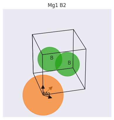
fbnc_kpath.structure.plot();
To plot the k-points belonging to the path:
fbnc_kpath.ebands.kpoints.plotly();
To plot the electronic fatbands grouped by atomic type:
fbnc_kpath.plot_fatbands_typeview(tight_layout=True);
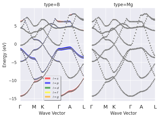
fbnc_kpath.plotly_fatbands_typeview();
To plot the electronic fatbands grouped by \(l\):
fbnc_kpath.plot_fatbands_lview(tight_layout=True);
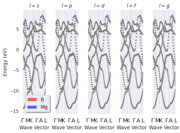
fbnc_kpath.plotly_fatbands_lview();
Now we read another FATBANDS.nc file produced on the 18x18x18 k-mesh
fbnc_kmesh = abilab.abiopen(abidata.ref_file("mgb2_kmesh181818_FATBANDS.nc"))
print(fbnc_kpath)
================================= File Info =================================
Name: mgb2_kpath_FATBANDS.nc
Directory: /home/runner/work/abipy_book/abipy_book/abipy/abipy/data/refs/mgb2_fatbands
Size: 149.01 kB
Access Time: Thu Jan 15 12:18:23 2026
Modification Time: Thu Jan 15 12:15:09 2026
Change Time: Thu Jan 15 12:15:09 2026

================================= Structure =================================
Full Formula (Mg1 B2)
Reduced Formula: MgB2
abc   :   3.086000   3.086000   3.523000
angles:  90.000000  90.000000 120.000000
pbc   :       True       True       True
Sites (3)
  #  SP           a         b    c
---  ----  --------  --------  ---
  0  Mg    0         0         0
  1  B     0.333333  0.666667  0.5
  2  B     0.666667  0.333333  0.5

Abinit Spacegroup: spgid: 191, num_spatial_symmetries: 24, has_timerev: True, symmorphic: False

============================== Electronic Bands ==============================
================================= Structure =================================
Full Formula (Mg1 B2)
Reduced Formula: MgB2
abc   :   3.086000   3.086000   3.523000
angles:  90.000000  90.000000 120.000000
pbc   :       True       True       True
Sites (3)
  #  SP           a         b    c
---  ----  --------  --------  ---
  0  Mg    0         0         0
  1  B     0.333333  0.666667  0.5
  2  B     0.666667  0.333333  0.5

Abinit Spacegroup: spgid: 191, num_spatial_symmetries: 24, has_timerev: True, symmorphic: False

Number of electrons: 8.0, Fermi level: 8.700 (eV)
nsppol: 1, nkpt: 78, mband: 8, nspinor: 1, nspden: 1
smearing scheme: none (occopt 1), tsmear_eV: 0.272, tsmear Kelvin: 3157.7
Direct gap:
    Energy: 0.595 (eV)
    Initial state: spin: 0, kpt: [+0.350, +0.300, +0.000], band: 3, eig: 8.402, occ: 2.000
    Final state:   spin: 0, kpt: [+0.350, +0.300, +0.000], band: 4, eig: 8.997, occ: 0.000
Fundamental gap:
    Energy: 0.058 (eV)
    Initial state: spin: 0, kpt: K [+0.333, +0.333, +0.000], band: 4, eig: 8.700, occ: 0.000
    Final state:   spin: 0, kpt: [+0.147, +0.000, +0.000], band: 4, eig: 8.758, occ: 0.000
Bandwidth: 14.314 (eV)
Valence maximum located at kpt index 27:
    spin: 0, kpt: K [+0.333, +0.333, +0.000], band: 4, eig: 8.700, occ: 0.000
Conduction minimum located at kpt index 5:
    spin: 0, kpt: [+0.147, +0.000, +0.000], band: 4, eig: 8.758, occ: 0.000

TIP: Use `--verbose` to print k-point coordinates with more digits

=============================== Fatbands Info ===============================
prtdos: 3, prtdosm: 0, mbesslang: 5, pawprtdos: 0, usepaw: 0
nsppol: 1, nkpt: 78, mband: 8

  Idx  Symbol    Reduced_Coords             Lmax    Ratsph [Bohr]  Has_Atom
-----  --------  -----------------------  ------  ---------------  ----------
    0  Mg        0.00000 0.00000 0.00000       4                2  Yes
    1  B         0.33333 0.66667 0.50000       4                2  Yes
    2  B         0.66667 0.33333 0.50000       4                2  Yes
and plot the \(l\)-PJDOS grouped by atomic type:
fbnc_kmesh.plot_pjdos_typeview(tight_layout=True);
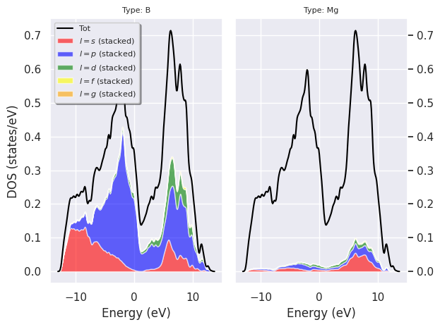
fbnc_kmesh.plotly_pjdos_typeview();
Plot the L-PJDOS grouped by L:
fbnc_kmesh.plot_pjdos_lview(tight_layout=True);
fbnc_kmesh.plotly_pjdos_lview();
Now we use the two netcdf files to produce plots with fatbands with PJDOSEs. The data for the DOS is taken from pjdosfile.
fbnc_kpath.plot_fatbands_with_pjdos(pjdosfile=fbnc_kmesh, view="type", tight_layout=True);
fbnc_kpath.plotly_fatbands_with_pjdos(pjdosfile=fbnc_kmesh, view="type");
fatbands plut PJDOS grouped by L:
fbnc_kpath.plot_fatbands_with_pjdos(pjdosfile=fbnc_kmesh, view="lview", tight_layout=True);
fbnc_kpath.plotly_fatbands_with_pjdos(pjdosfile=fbnc_kmesh, view="lview");
Warning
Remember to close the files with:
fbnc_kpath.close()
fbnc_kmesh.close()