The HIST.nc file (relaxation/MD)#
The HIST.nc file contains the history of structural relaxations or molecular dynamics calculations.
One can use the abiopen function provide by abilab to open the file and generate an instance of HistFile.
Alteratively, one can use the abiopen.py script to open the file inside the shell with the syntax:
abiopen.py out_HIST.nc
This command will start the ipython interpreter so that one can interact directly
with the HistFile object (named abifile inside ipython).
To generate a jupyter notebook use:
abiopen.py out_HIST.nc -nb
For a quick visualization of the data, use the --expose option:
abiopen.py out_HIST.nc -e
import warnings
warnings.filterwarnings("ignore")  # Ignore warnings

from abipy import abilab
abilab.enable_notebook() # This line tells AbiPy we are running inside a notebook
import abipy.data as abidata

# This line configures matplotlib to show figures embedded in the notebook.
# Replace `inline` with `notebook` in classic notebook
%matplotlib inline

# Option available in jupyterlab. See https://github.com/matplotlib/jupyter-matplotlib
#%matplotlib widget
hist = abilab.abiopen(abidata.ref_file("sic_relax_HIST.nc"))
print("Number of iterations performed:", hist.num_steps)
Number of iterations performed: 7
hist.structures is the list of structure objects at the different iteration steps.
hist.etotals is a numpy array with the total energies in eV associated to the different steps.
for struct, etot in zip(hist.structures, hist.etotals):
    print("Volume:", struct.volume,", Etotal:", etot)
Volume: 20.35143850388187 , Etotal: -285.4877026790871
Volume: 20.409158438655506 , Etotal: -285.4890033792876
Volume: 20.383305112143578 , Etotal: -285.48909437441085
Volume: 20.3569371210443 , Etotal: -285.48912759682247
Volume: 20.356014923020417 , Etotal: -285.48912778072355
Volume: 20.3517927586343 , Etotal: -285.48912733499026
Volume: 20.355222198448786 , Etotal: -285.48912780554605
To get the last structure stored in the HIST.nc file:
print(hist.final_structure)
Full Formula (Si1 C1)
Reduced Formula: SiC
abc   :   3.064763   3.064763   3.064763
angles:  60.000000  60.000000  60.000000
pbc   :       True       True       True
Sites (2)
  #  SP        a     b      c  cartesian_forces
---  ----  -----  ----  -----  -----------------------
  0  C     -0     0     -0     [-0. -0. -0.] eV ang^-1
  1  Si     0.25  0.25   0.25  [-0. -0. -0.] eV ang^-1
min |F_iat|: 0.0 eV/Ang
max |F_iat|: 0.0 eV/Ang
mean F_iat|: 0.0 eV/Ang
std  |F_iat|: 0.0 eV/Ang
Forces are relaxed within high quality criterion: 0.0001 eV/Ang
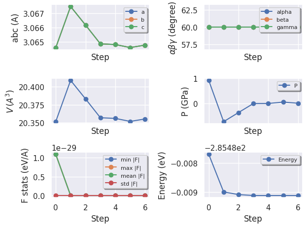
To plot the evolution of the structural parameters with matplotlib:
hist.plot(tight_layout=True);

hist.plotly();
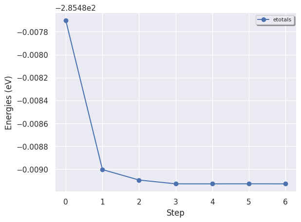
To plot the total energies at the different iterations steps:
hist.plot_energies();

hist.plotly_energies();
Converting to other formats#
Use to_xdatcar to get a XDATCAR pymatgen object (useful to interface AbiPy with other pymatgen tools)
# hist.write_xdatcar writes a XDATCAR file
xdatcar = hist.to_xdatcar()
print(xdatcar)
Si1 C1
1.0
0.000000 2.166981 2.166981
2.166981 0.000000 2.166981
2.166981 2.166981 0.000000
C Si
1 1
Direct configuration=      1
0.00000000 0.00000000 0.00000000
0.25000000 0.25000000 0.25000000
Direct configuration=      2
-0.00000000 0.00000000 -0.00000000
0.25000000 0.25000000 0.25000000
Direct configuration=      3
-0.00000000 0.00000000 -0.00000000
0.25000000 0.25000000 0.25000000
Direct configuration=      4
-0.00000000 0.00000000 -0.00000000
0.25000000 0.25000000 0.25000000
Direct configuration=      5
-0.00000000 0.00000000 -0.00000000
0.25000000 0.25000000 0.25000000
Direct configuration=      6
-0.00000000 0.00000000 -0.00000000
0.25000000 0.25000000 0.25000000
Direct configuration=      7
-0.00000000 0.00000000 -0.00000000
0.25000000 0.25000000 0.25000000

