The MDF file (Bethe-Salpeter)#
The Bethe-Salpeter code saves the optical spectra in the MDF.nc file.
This notebook explains how to use the AbiPy API to analyze the results.
Let’s start by importing the basic modules we will need for this tutorial.
import warnings
warnings.filterwarnings("ignore")  # Ignore warnings

from abipy import abilab
abilab.enable_notebook() # This line tells AbiPy we are running inside a notebook
import abipy.data as abidata

# This line configures matplotlib to show figures embedded in the notebook.
# Replace `inline` with `notebook` in classic notebook
%matplotlib inline

# Option available in jupyterlab. See https://github.com/matplotlib/jupyter-matplotlib
#%matplotlib widget
How to analyze a single MDF file#
Use abiopen to open the MDF:
mdf_file = abilab.abiopen(abidata.ref_file("tbs_4o_DS2_MDF.nc"))
print(mdf_file)
================================= File Info =================================
Name: tbs_4o_DS2_MDF.nc
Directory: /home/runner/work/abipy_book/abipy_book/abipy/abipy/data/refs/si_bse
Size: 104.53 kB
Access Time: Thu Jan 15 12:20:31 2026
Modification Time: Thu Jan 15 12:15:09 2026
Change Time: Thu Jan 15 12:15:09 2026

================================= Structure =================================
Full Formula (Si2)
Reduced Formula: Si
abc   :   3.823046   3.823046   3.823046
angles:  60.000000  60.000000  60.000000
pbc   :       True       True       True
Sites (2)
  #  SP       a     b     c
---  ----  ----  ----  ----
  0  Si    0     0     0
  1  Si    0.25  0.25  0.25

Abinit Spacegroup: spgid: 0, num_spatial_symmetries: 48, has_timerev: True, symmorphic: True
================================== Q-points ==================================
0) [+0.939, +0.000, +0.000]
1) [+0.000, +0.939, +0.000]
2) [+0.000, +0.000, +0.939]
3) [+0.000, +0.813, +0.813]
4) [+0.813, +0.000, +0.813]
5) [+0.813, +0.813, +0.000]
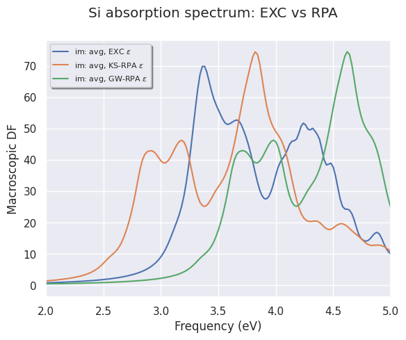
To plot the (averaged) imaginary part of the macroscopic dielectric function (MDF) between 2 and 5 eV use:
mdf_file.plot_mdfs(title="Si absorption spectrum: EXC vs RPA", xlims=(2, 5));
To select the MDF computed for the first q-point, use
mdf_file.plot_mdfs(title="Im(Mdf) at the first q-point", qpoint=0, xlims=(2, 5));
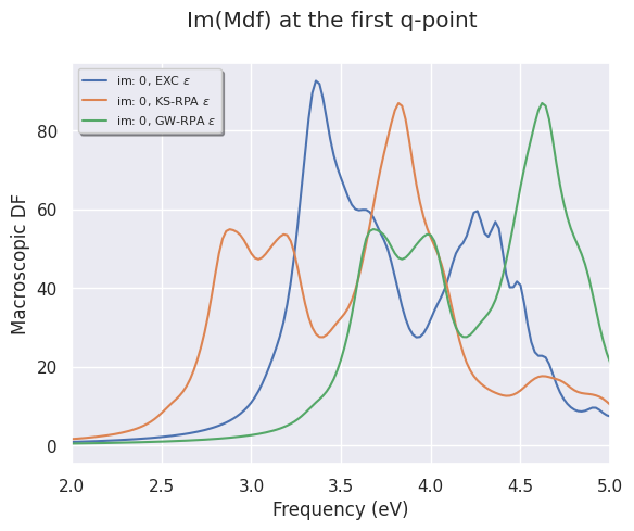
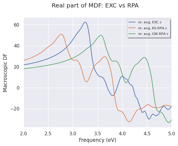
EXC: MDF with excitonic effects included
KS-RPA: MDF computed with KS eigenvalues
GW-RPA: MDF computed at the RPA level with KS + scissors operator
To plot the (averaged) real part of the MDF:
mdf_file.plot_mdfs(cplx_mode="re", title="Real part of MDF: EXC vs RPA", xlims=(2, 5));
Analyzing multiple MDF files with robots#
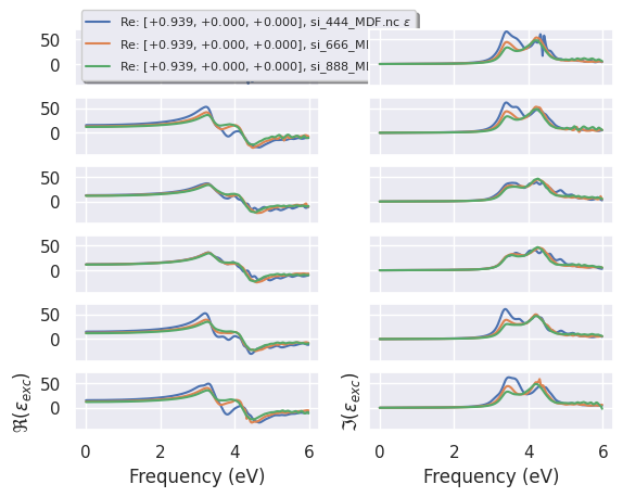
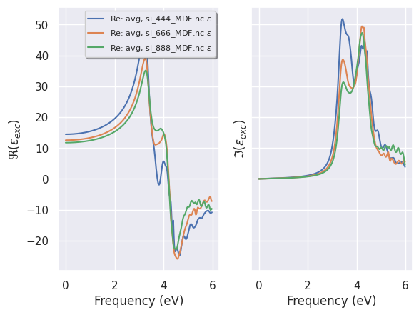
To analyze the converge of the optical spectra, we can use the MdfRobot. Let’s build our robot from a list of MDF.nc files:
paths = abidata.ref_files("si_444_MDF.nc", "si_666_MDF.nc", "si_888_MDF.nc")
robot = abilab.MdfRobot.from_files(paths)
print(robot)
MdfRobot with 3 files in memory:

================================= File Info =================================
Name: si_444_MDF.nc
Directory: /home/runner/work/abipy_book/abipy_book/abipy/abipy/data/refs/si_bse_kpoints
Size: 102.53 kB
Access Time: Thu Jan 15 12:20:32 2026
Modification Time: Thu Jan 15 12:15:09 2026
Change Time: Thu Jan 15 12:15:09 2026

================================= Structure =================================
Full Formula (Si2)
Reduced Formula: Si
abc   :   3.823046   3.823046   3.823046
angles:  60.000000  60.000000  60.000000
pbc   :       True       True       True
Sites (2)
  #  SP       a     b     c
---  ----  ----  ----  ----
  0  Si    0     0     0
  1  Si    0.25  0.25  0.25

Abinit Spacegroup: spgid: 0, num_spatial_symmetries: 48, has_timerev: True, symmorphic: True
================================== Q-points ==================================
0) [+0.939, +0.000, +0.000]
1) [+0.000, +0.939, +0.000]
2) [+0.000, +0.000, +0.939]
3) [+0.000, +0.813, +0.813]
4) [+0.813, +0.000, +0.813]
5) [+0.813, +0.813, +0.000]


================================= File Info =================================
Name: si_666_MDF.nc
Directory: /home/runner/work/abipy_book/abipy_book/abipy/abipy/data/refs/si_bse_kpoints
Size: 122.71 kB
Access Time: Thu Jan 15 12:20:32 2026
Modification Time: Thu Jan 15 12:15:09 2026
Change Time: Thu Jan 15 12:15:09 2026

================================= Structure =================================
Full Formula (Si2)
Reduced Formula: Si
abc   :   3.823046   3.823046   3.823046
angles:  60.000000  60.000000  60.000000
pbc   :       True       True       True
Sites (2)
  #  SP       a     b     c
---  ----  ----  ----  ----
  0  Si    0     0     0
  1  Si    0.25  0.25  0.25

Abinit Spacegroup: spgid: 0, num_spatial_symmetries: 48, has_timerev: True, symmorphic: True
================================== Q-points ==================================
0) [+0.939, +0.000, +0.000]
1) [+0.000, +0.939, +0.000]
2) [+0.000, +0.000, +0.939]
3) [+0.000, +0.813, +0.813]
4) [+0.813, +0.000, +0.813]
5) [+0.813, +0.813, +0.000]


================================= File Info =================================
Name: si_888_MDF.nc
Directory: /home/runner/work/abipy_book/abipy_book/abipy/abipy/data/refs/si_bse_kpoints
Size: 162.03 kB
Access Time: Thu Jan 15 12:20:32 2026
Modification Time: Thu Jan 15 12:15:09 2026
Change Time: Thu Jan 15 12:15:09 2026

================================= Structure =================================
Full Formula (Si2)
Reduced Formula: Si
abc   :   3.823046   3.823046   3.823046
angles:  60.000000  60.000000  60.000000
pbc   :       True       True       True
Sites (2)
  #  SP       a     b     c
---  ----  ----  ----  ----
  0  Si    0     0     0
  1  Si    0.25  0.25  0.25

Abinit Spacegroup: spgid: 0, num_spatial_symmetries: 48, has_timerev: True, symmorphic: True
================================== Q-points ==================================
0) [+0.939, +0.000, +0.000]
1) [+0.000, +0.939, +0.000]
2) [+0.000, +0.000, +0.939]
3) [+0.000, +0.813, +0.813]
4) [+0.813, +0.000, +0.813]
5) [+0.813, +0.813, +0.000]
plotter = robot.get_multimdf_plotter()
To analyze the convergence of the (averaged) MDFs:
plotter.plot();
It is also possible to analyze the converge of the MDF for the different q-directions with:
plotter.plot(qview="all");
