LumiWork Workflow#
This tutorial aims to show how to perform \(\Delta\)SCF constrained-occupations computations with Abinit in an automated way. The theory and equations associated to this tutorial can be found in the related theory section, and references therein.
Note
Before starting, it is recommended to first get familiar with the AbiPy environment, in particular the working principle of AbiPy workflows.
Note
The examples shown in these tutorials are based on a certain type of defect (Eu substitution), but the \(\Delta\)SCF constrained-occupations methodology can be applied to numerous kind of defects.
Recap#
Our goal is to compute the photo-luminescent properties of an impurity embedded in a lattice. Here we will take the example of the red phosphor material Sr[Li\(_2\)Al\(_2\)O\(_2\)N\(_2\)]:Eu\(^{2+}\).
We need to compute the four states (energies and structures) highlighted in the figure below:
Relaxed ground state (A\(_g\))
Unrelaxed excited state (A\(_{e}^{*}\))
Relaxed excited state (A\(_{e}\))
Unrelaxed ground state (A\(_{g}^{*}\))
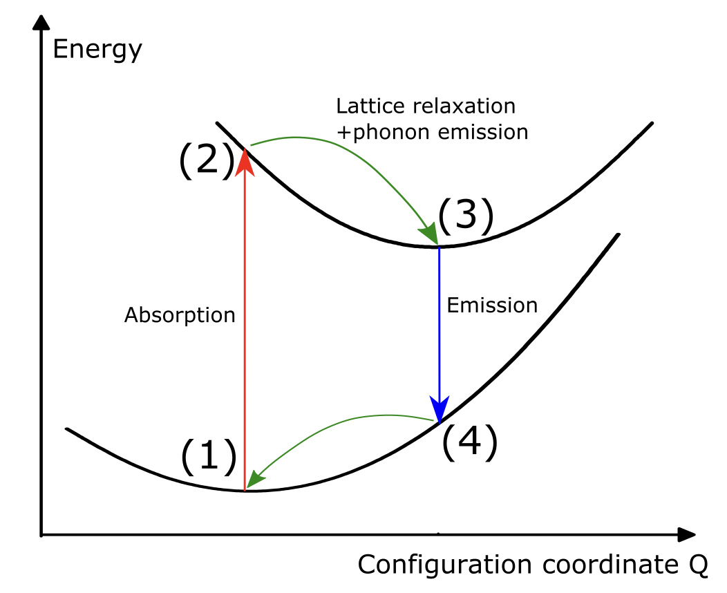
This requires two relaxations (one in the ground and excited state) and four static scf computations (at each state). One could eventually add four nscf computations for the electronic band structures. These 6 (+4) computations are what is automatized in one “LumiWork”.
The excited state configuration is computed following the \(\Delta\)SCF-constrained occupation method.
A key challenge in \(\Delta\)SCF calculations is correctly setting up the occupation numbers for both ground and excited states.
General Principles#
For a spin-polarized calculation (nsppol=2), you need to specify occupations separately for spin-up and spin-down channels with the occ input variable in Abinit.
For instance, it might read like for the ground state :
N_occ_el_up*1  N_empty_el_up*0
N_occ_el_dn*1  N_empty_el_dn*0
where N_occ_el_up and N_occ_el_dn are the number of occupied bands for spin-up and spin-down channels, respectively, and N_empty_el_up and N_empty_el_dn are the number of empty (conduction) bands.
For the excited state, we can create a “hole” in the highest occupied state and promote one electron to the lowest unoccupied state:
(N_occ_el_up-1)*1  0  1  (N_empty_el_up-1)*0
N_occ_el_dn*1  N_empty_el_dn*0
This pattern needs to be adapted based on:
The total number of valence electrons in your system
The electronic configuration of your defect
The type of excitation (e.g., d-d, f-d, spin-flip)
LumiWork Workflow#
Note
The example shown in this tutorial is designed to run in a few minutes on a laptop, meaning that the results are unconverged (supercell size, different DFT parameters,…). Results of production runs for this kind of system can be found in references [Bouquiaux et al., 2021] and [Bouquiaux et al., 2023]
The creation of one LumiWork is done with the class method from_scf_inputs():
from abipy.flowtk.lumi_works import LumiWork
help(LumiWork.from_scf_inputs)
Help on method from_scf_inputs in module abipy.flowtk.lumi_works:

from_scf_inputs(gs_scf_inp, ex_scf_inp, relax_kwargs_gs, relax_kwargs_ex, ndivsm=0, nb_extra=10, tolwfr=1e-12, four_points=True, meta=None, manager=None) -> 'LumiWork' class method of abipy.flowtk.lumi_works.LumiWork
    Args:
        gs_scf_inp: |AbinitInput| representing a GS SCF run for the ground-state.
        ex_scf_inp: |AbinitInput| representing a GS SCF run for the excited-state.
        relax_kwargs_gs: Dictonary with input variables to be added to gs_scf_inp
            when generating input files for ground state structural relaxations.
        relax_kwargs_ex: Dictonary with input variables to be added to ex_scf_inp
            when generating input files for excited state structural relaxations.
        ndivsm: Activates the computation of band structure if different from zero.
            if > 0, it's the number of divisions for the smallest segment of the path (Abinit variable).
            if < 0, it's interpreted as the pymatgen `line_density` parameter in which the number of points
            in the segment is proportional to its length. Typical value: -20.
            This option is the recommended one if the k-path contains two high symmetry k-points that are very close
            as ndivsm > 0 may produce a very large number of wavevectors.
        nb_extra: Number of extra bands added to the input nband when computing band structures (ndivsm != 0).
        tolwfr: Tolerance of the residuals used for the NSCF band structure calculations.
        four_points: if True, compute the two relaxations and the four points energies.
            If false, only the two relaxations.
        meta: dict corresponding to the metadata of a lumiwork (supercell size, dopant type,...)
        manager: |TaskManager| of the task. If None, the manager is initialized from the config file.
This class method is a container that receives mainly Abinit Input objects and dictionnaries of Abinit variables.
The lumi_works.py script will then use these informations to do the following tasks:
Launch a first structural relaxation in the ground state (task t0), save the ground-state relaxed structure.
Use the previous structure as the starting point for a second structural relaxation in the excited state (task t1), save the excited-state relaxed structure.
Launch the four static scf tasks simultaneously (tasks t2, t3, t4 and t5 in the order shown in the recap section)
Launch optionnaly the four NSCF tasks (tasks t6, t7, t8 and t9 in the same order)
Perform a first quick post-process and store the results in
flow_deltaSCF/w0/outdata/Delta_SCF.json.
Creating a LumiWork#
Note
The complete workflow was ran separately, before building this jupyter book. You will find the worflow scripts and corresponding folder here.
A LumiWork (or a serie of LumiWork’s) can be created with the run_deltaSCF.py script, as shown below:
#!/usr/bin/env python
import sys
import os
import abipy.abilab as abilab
import abipy.flowtk as flowtk
import abipy.data as abidata
from abipy.core import structure

def scf_inp(structure):
    pseudodir = 'pseudos'

    pseudos = ('Eu.xml',
               'Sr.xml',
               'Al.xml',
               'Li.xml',
               'O.xml',
               'N.xml')

    gs_scf_inp = abilab.AbinitInput(structure=structure, pseudos=pseudos, pseudo_dir=pseudodir)
    gs_scf_inp.set_vars(ecut=10,
                        pawecutdg=20,
                        chksymbreak=0,
                        diemac=5,
                        prtwf=-1,
                        nstep=100,
                        toldfe=1e-6,
                        chkprim=0,
                        )

    # Set DFT+U and spinat parameters according to chemical symbols.
    symb2spinat = {"Eu": [0, 0, 7]}
    symb2luj = {"Eu": {"lpawu": 3, "upawu": 7, "jpawu": 0.7}}

    gs_scf_inp.set_usepawu(usepawu=1, symb2luj=symb2luj)
    gs_scf_inp.set_spinat_from_symbols(symb2spinat, default=(0, 0, 0))

    n_val = gs_scf_inp.num_valence_electrons
    n_cond = round(20)

    spin_up_gs = f"\n{int((n_val - 7) / 2)}*1 7*1 {n_cond}*0"
    spin_up_ex = f"\n{int((n_val - 7) / 2)}*1 6*1 0 1 {n_cond - 1}*0"
    spin_dn = f"\n{int((n_val - 7) / 2)}*1 7*0 {n_cond}*0"

    nsppol = 2
    shiftk = [0, 0, 0]
    ngkpt = [1, 1, 1]

    # Build SCF input for the ground state configuration.
    gs_scf_inp.set_kmesh_nband_and_occ(ngkpt, shiftk, nsppol, [spin_up_gs, spin_dn])

    # Build SCF input for the excited configuration.
    exc_scf_inp = gs_scf_inp.deepcopy()
    exc_scf_inp.set_kmesh_nband_and_occ(ngkpt, shiftk, nsppol, [spin_up_ex, spin_dn])

    return gs_scf_inp,exc_scf_inp


def relax_kwargs():

    # Dictionary with input variables to be added for performing structural relaxations.
    relax_kwargs = dict(
        ecutsm=0.5,
        toldff=1e-4, # TOO HIGH, just for testing purposes.
        tolmxf=1e-3, # TOO HIGH, just for testing purposes.
        ionmov=2,
        dilatmx=1.05,  # Keep this also for optcell 0 else relaxation goes bananas due to low ecut.
        chkdilatmx=0,
    )

    relax_kwargs_gs=relax_kwargs.copy()
    relax_kwargs_gs['optcell'] = 0 # in the ground state, if allow relaxation of the cell (optcell 2)

    relax_kwargs_ex=relax_kwargs.copy()
    relax_kwargs_ex['optcell'] = 0 # in the excited state, no relaxation of the cell

    return relax_kwargs_gs, relax_kwargs_ex


def build_flow(options):

    # Working directory (default is the name of the script with '.py' removed and "run_" replaced by "flow_")
    if not options.workdir:
        options.workdir = os.path.basename(sys.argv[0]).replace(".py", "").replace("run_", "flow_")

    flow = flowtk.Flow(options.workdir, manager=options.manager)

    # Construct the structures
    prim_structure = structure.Structure.from_file('SALON_prim.cif')
    structure_list = prim_structure.make_doped_supercells([1,1,2], 'Sr', 'Eu')

    ####### Delta SCF part of the flow #######

    from abipy.flowtk.lumi_works import LumiWork

    for stru in structure_list:
       gs_scf_inp, exc_scf_inp = scf_inp(stru)
       relax_kwargs_gs, relax_kwargs_ex = relax_kwargs()
       Lumi_work = LumiWork.from_scf_inputs(gs_scf_inp, exc_scf_inp, relax_kwargs_gs, relax_kwargs_ex,ndivsm=0)
       flow.register_work(Lumi_work)

    return flow


@flowtk.flow_main
def main(options):
    """
    This is our main function that will be invoked by the script.
    flow_main is a decorator implementing the command line interface.
    Command line args are stored in `options`.
    """
    return build_flow(options)


if __name__ == '__main__':
    sys.exit(main())
Let’s decompose this script.
We first create the abinit input objects.
This is achieved by the function def scf_inp(structure): that takes as argument a structure object.
It returns abinit input objects for the ground and excited state.
It is in this function that all the important abinit variables that are specific to the system under study are located.
The tricky part is the automatic definition of the occupation numbers. Let’s break down the Eu\(^{2+}\) example step by step:
    n_val = gs_scf_inp.num_valence_electrons  # Total valence electrons in the supercell
    n_cond = round(20)  # Number of conduction bands to include (user choice)

    #### SPECIFIC to Eu2+ doped system (7 electrons in 4f shell) ####
    spin_up_gs = f"\n{int((n_val - 7) / 2)}*1 7*1 {n_cond}*0"
    spin_up_ex = f"\n{int((n_val - 7) / 2)}*1 6*1 0 1 {n_cond - 1}*0"
    spin_dn = f"\n{int((n_val - 7) / 2)}*1 7*0 {n_cond}*0"
    ####################################################################

    nsppol = 2
    shiftk = [0, 0, 0]
    ngkpt = [1, 1, 1]

    # Build SCF input for the ground state configuration.
    gs_scf_inp.set_kmesh_nband_and_occ(ngkpt, shiftk, nsppol, [spin_up_gs, spin_dn])

    # Build SCF input for the excited configuration.
    exc_scf_inp = gs_scf_inp.deepcopy()
    exc_scf_inp.set_kmesh_nband_and_occ(ngkpt, shiftk, nsppol, [spin_up_ex, spin_dn])
Note
Eu\(^{2+}\) has the electronic configuration [Xe]4f\(^7\)5d\(^0\). In the ground state, the seven 4f electrons are all spin-up (due to Hund’s rules). The excited state corresponds to a 4f\(\rightarrow\)5d transition: one 4f electron is promoted to the 5d shell.
Let’s decompose the occupation strings:
spin_up_gs: Ground state, spin-up channel
{int((n_val - 7) / 2)}*1: All “normal” valence electrons (excluding Eu 4f) \(\rightarrow\) fully occupied7*1: The seven 4f electrons of Eu\(^{2+}\) \(\rightarrow\) fully occupied{n_cond}*0: Empty conduction bands
spin_up_ex: Excited state, spin-up channel
{int((n_val - 7) / 2)}*1: All “normal” valence electrons \(\rightarrow\) still fully occupied6*1: Only six 4f electrons remain \(\rightarrow\) occupied0: One empty 4f state (the “hole”)1: One electron promoted to 5d \(\rightarrow\) occupied{n_cond - 1}*0: Remaining conduction bands empty
spin_dn: Spin-down channel (identical for ground and excited states)
{int((n_val - 7) / 2)}*1: All “normal” valence electrons \(\rightarrow\) occupied7*0: No spin-down 4f electrons{n_cond}*0: Empty conduction bands
Why \((n_{val} - 7) / 2\)?
This counts all valence electrons except the 7 Eu 4f electrons. We divide by 2 because in the spin-polarized calculation, these “normal” electrons are equally distributed between spin-up and spin-down channels.
A further example is presented for a spin-flip transition at the the end of this page.
The relaxation parameters (that might be different between ground and excited state!) are given in the function def relax_kwargs():.
Finally, we are now able to create the workflow with:
def build_flow(options):

    # Working directory (default is the name of the script with '.py' removed and "run_" replaced by "flow_")
    if not options.workdir:
        options.workdir = os.path.basename(sys.argv[0]).replace(".py", "").replace("run_", "flow_")

    flow = flowtk.Flow(options.workdir, manager=options.manager)

    # Construct the structures
    prim_structure = structure.Structure.from_file('SALON_prim.cif')
    structure_list = prim_structure.make_doped_supercells([1,1,2], 'Sr', 'Eu')

    ####### Delta SCF part of the flow #######

    from abipy.flowtk.lumi_works import LumiWork

    for stru in structure_list: ## loop through all the non-equivalent sites available for Eu.
       gs_scf_inp, exc_scf_inp = scf_inp(stru)
       relax_kwargs_gs, relax_kwargs_ex = relax_kwargs()
       Lumi_work = LumiWork.from_scf_inputs(gs_scf_inp, exc_scf_inp, relax_kwargs_gs, relax_kwargs_ex,ndivsm=0)
       flow.register_work(Lumi_work)

    return flow
Where we have use the convenient make_doped_supercells() method.
from abipy.core.structure import Structure
help(Structure.make_doped_supercells)
Help on function make_doped_supercells in module abipy.core.structure:

make_doped_supercells(self, scaling_matrix, replaced_atom: 'str', dopant_atom: 'str') -> 'list[Structure]'
    Returns a list of doped supercell structures, one for each non-equivalent site of the replaced atom.

    Args:
        scaling_matrix: A scaling matrix for transforming the lattice vectors.
            Has to be all integers. Several options are possible:
            a) A full 3x3 scaling matrix defining the linear combination of the old lattice vectors.
            E.g., [[2,1,0],[0,3,0],[0,0,1]] generates a new structure with lattice vectors
            a_new = 2a + b, b_new = 3b, c_new = c
            where a, b, and c are the lattice vectors of the original structure.
            b) A sequence of three scaling factors. e.g., [2, 1, 1]
            specifies that the supercell should have dimensions 2a x b x c.
            c) A number, which simply scales all lattice vectors by the same factor.
        replaced atom: Symbol of the atom to be replaced (ex: 'Sr')
        dopant_atom: Symbol of the dopant_atom (ex: 'Eu')
Running a LumiWork#
Let us run see what running the code in practice looks like. In your terminal, create the worfklow with
python run_deltaSCF.py
A new /flow_deltaSCF folder should be created.
We observe that at this time, only one taks is created in /flow_deltaSCF/w0/t0, the first ground state relaxation.
This is normal since the rest of the workflow will be created at run-time, when the ground state relaxed structure will be extracted.
We launch the flow with the command:
nohup abirun.py flow_deltaSCF scheduler > log 2> err &
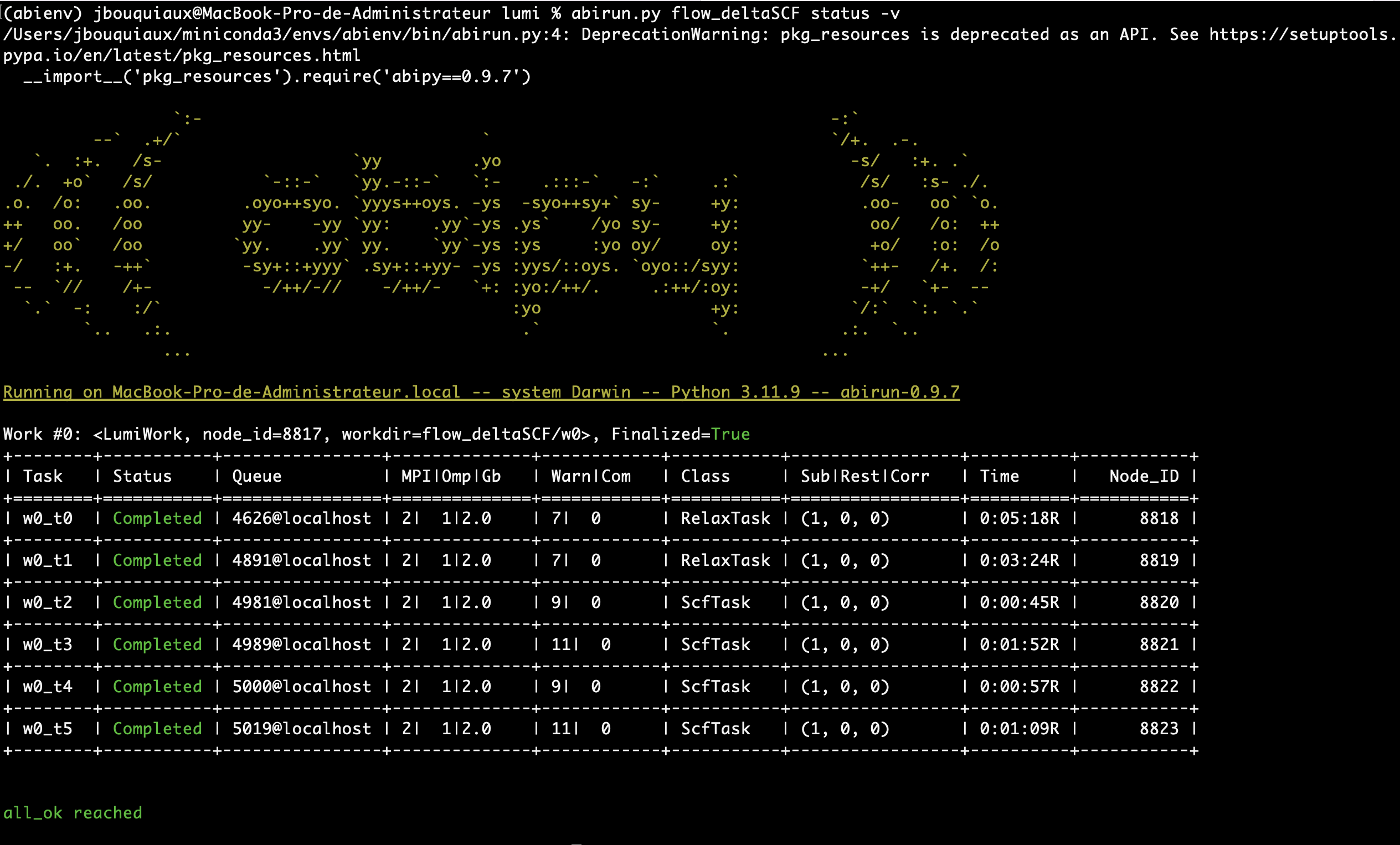
After completion, you can verify the status of the flow with
abirun.py flow_deltaSCF status
A first quick post-processing of the results (following a 1D-CCM, see next section)
can be found in /flow_deltaSCF/w0/Delta_SCF.json file.
Relaxations only?#
In some cases, it might be interesting to perform the two relaxations only, or the 4 static computations only.
This flexibility is allowed thanks to the LumiWork_relaxations() class
from abipy.flowtk.lumi_works import LumiWork_relaxations

print(LumiWork_relaxations.__doc__)
help(LumiWork_relaxations.from_scf_inputs)
    This Work implements the ground and excited state relaxations only.

    The relaxations run simultaneously. No task creation at run-time.

Help on method from_scf_inputs in module abipy.flowtk.lumi_works:

from_scf_inputs(gs_scf_inp, ex_scf_inp, relax_kwargs_gs, relax_kwargs_ex, meta=None, manager=None) class method of abipy.flowtk.lumi_works.LumiWork_relaxations
    Args:
        gs_scf_inp: |AbinitInput| representing a GS SCF run for the ground-state.
        ex_scf_inp: |AbinitInput| representing a GS SCF run for the excited-state.
        relax_kwargs_gs: Dictonary with input variables to be added to gs_scf_inp
            when generating input files for ground state structural relaxations.
        relax_kwargs_ex: Dictonary with input variables to be added to ex_scf_inp
            when generating input files for excited state structural relaxations.
        meta: dict corresponding to the metadata of a lumiwork (supercell size, dopant type,...)
        manager: |TaskManager| of the task. If None, the manager is initialized from the config file.
and with the LumiWorkFromRelax class
from abipy.flowtk.lumi_works import LumiWorkFromRelax

print(LumiWorkFromRelax.__doc__)
help(LumiWorkFromRelax.from_scf_inputs)
    Same as LumiWork, without the relaxations. Typically used after a LumiWork_relaxations work.
    The two relaxed structures (in ground and excited state) are given as input. No creation at run-time


Help on method from_scf_inputs in module abipy.flowtk.lumi_works:

from_scf_inputs(gs_scf_inp, ex_scf_inp, gs_structure, ex_structure, ndivsm=0, nb_extra=10, tolwfr=1e-12, meta=None, manager=None) class method of abipy.flowtk.lumi_works.LumiWorkFromRelax
    Args:
        gs_scf_inp: |AbinitInput| representing a GS SCF run for the ground-state.
        exc_scf_inp: |AbinitInput| representing a GS SCF run for the excited-state.
        gs_structure: object representing the relaxed ground state structure
        ex_structure: object representing the excited ground state structure
        ndivsm: Activates the computation of band structure if different from zero.
            if > 0, it's the number of divisions for the smallest segment of the path (Abinit variable).
            if < 0, it's interpreted as the pymatgen `line_density` parameter in which the number of points
            in the segment is proportional to its length. Typical value: -20.
            This option is the recommended one if the k-path contains two high symmetry k-points that are very close
            as ndivsm > 0 may produce a very large number of wavevectors.
        nb_extra: Number of extra bands added to the input nband when computing band structures (ndivsm != 0).
        tolwfr: Tolerance of the residuals used for the NSCF band structure calculations.
        manager: |TaskManager| of the task. If None, the manager is initialized from the config file.
Running only one computation is also feasible by changing the end of the run_DeltaSCF.py script.
For example, if you only need the ground state relaxation, you might use LumiWork_relaxations.from_scf_inputs()
and register only the first task:
Lumi_work = LumiWork_relaxations.from_scf_inputs(gs_scf_inp, exc_scf_inp, relax_kwargs_gs, relax_kwargs_ex,ndivsm=0)

flow.register_task(Lumi_work[0]) # notice the register_task and not register_work
Additional Example: F-center in CaO#
Background#
An F-center is a neutral oxygen vacancy with two trapped electrons. Unlike the Eu\(^{2+}\) case where we have a 4f\(\rightarrow\)5d electron promotion, the F-center excited state results from a spin-flip transition: one electron flips from spin-down to spin-up, changing from a singlet to a triplet configuration.
Ground state: Two electrons with opposite spins in the defect state (singlet, \(S=0\))
Spin-up: 1 electron in defect state
Spin-down: 1 electron in defect state
Excited state: Both electrons have parallel spins (triplet, \(S=1\))
Spin-up: 2 electrons in defect state (one original + one flipped from spin-down)
Spin-down: 0 electrons in defect state
Occupation Setup#
The key part of the occupation setup for the F-center case:
def scf_inp_fcenter(structure):
    # ... (pseudopotentials, basic parameters)

    n_val = gs_scf_inp.num_valence_electrons
    n_cond = 4  # Number of conduction bands

    # For this example: 60 host valence electrons + 2 defect electrons
    n_host = 60

    #### SPECIFIC to F-center (2 electrons, spin-flip excitation) ####
    # Ground state: singlet configuration (one electron per spin channel)
    spin_up_gs = f"\n{n_host}*1 1 0 {n_cond}*0"  # 60 host + 1 defect electron
    spin_dn_gs = f"\n{n_host}*1 1 0 {n_cond}*0"  # 60 host + 1 defect electron

    # Excited state: triplet configuration (both electrons in spin-up)
    spin_up_ex = f"\n{n_host}*1 1 1 {n_cond-1}*0"  # 60 host + 2 defect electrons
    spin_dn_ex = f"\n{n_host}*1 0 0 {n_cond}*0"    # 60 host + 0 defect electrons
    ####################################################################

    nsppol = 2
    ngkpt = [1, 1, 1]
    shiftk = [0, 0, 0]

    # Build SCF input for ground state
    gs_scf_inp.set_kmesh_nband_and_occ(ngkpt, shiftk, nsppol, [spin_up_gs, spin_dn_gs])

    # Build SCF input for excited state
    exc_scf_inp = gs_scf_inp.deepcopy()
    exc_scf_inp.set_kmesh_nband_and_occ(ngkpt, shiftk, nsppol, [spin_up_ex, spin_dn_ex])

    return gs_scf_inp, exc_scf_inp
Tip
When adapting this workflow to your own defect system:
Identify the total number of valence electrons:
n_val = gs_scf_inp.num_valence_electronsDetermine how many electrons are localized on your defect
Understand the nature of the excitation (promotion vs. spin-flip vs. other)
Write appropriate occupation strings for each spin channel
Test with a small calculation to confirm the occupation pattern produces the expected electronic structure