The GSR file (Ground-State Results)#
In this notebook we discuss how to plot the electron band structures and the density of states (DOS) using the GSR netcdf files produced by Abinit.
For the tutorial, we will use the netcdf files shipped with AbiPy.
The function abidata.ref_file returns the absolute path of the reference file.
In your scripts, you have to replace data.ref_file("abipy_filename") with a string giving
the location of your netcdf file.
Alternatively, one can use the abiopen.py script to open the file inside the shell with the syntax:
abiopen.py out_GSR.nc
This command will start the ipython interpreter so that one can interact directly
with the GsrFile object (named abifile inside ipython).
To generate a jupyter notebook use:
abiopen.py out_GSR.nc -nb
For a quick visualization of the data, use the --expose options:
abiopen.py out_GSR.nc -e
Note
Simple visualization tasks can be easily automated by just issuing in the terminal:
abiopen.py FILE --expose
to generate a predefined list of matplotlib plots.
To activate the plotly version (if available) use:
abiopen.py FILE --plotly
Note also that one can generate jupyter-lab notebooks directly from the command line with abiopen.py and the command:
abiopen.py FILE -nb
Add --classic-notebook if you prefer classic jupyter notebooks.
Finally, use one of the options of the abiview.py script to plot the results automatically.
import warnings
warnings.filterwarnings("ignore")  # Ignore warnings

from abipy import abilab
abilab.enable_notebook() # This line tells AbiPy we are running inside a notebook
# Import abipy reference data.
import abipy.data as abidata

# This line configures matplotlib to show figures embedded in the notebook.
# Replace `inline` with `notebook` in classic notebook
%matplotlib inline

# Option available in jupyterlab. See https://github.com/matplotlib/jupyter-matplotlib
#%matplotlib widget
The GSR File#
The GSR file (mnemonics: Ground-State Results) is a netcdf file with the
results produced by SCF or NSCF ground-state calculations
(band energies, forces, energies, stress tensor).
To open a GSR file, use the abiopen function defined in abilab:
gsr = abilab.abiopen(abidata.ref_file("si_scf_GSR.nc"))
The gsr object has a Structure:
print(gsr.structure)
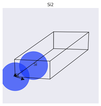
Full Formula (Si2)
Reduced Formula: Si
abc   :   3.866975   3.866975   3.866975
angles:  60.000000  60.000000  60.000000
pbc   :       True       True       True
Sites (2)
  #  SP       a     b     c  cartesian_forces
---  ----  ----  ----  ----  -----------------------------------------------------------
  0  Si    0     0     0     [-5.89948307e-27 -1.93366149e-27  2.91016904e-27] eV ang^-1
  1  Si    0.25  0.25  0.25  [ 5.89948307e-27  1.93366149e-27 -2.91016904e-27] eV ang^-1
min |F_iat|: 6.856532001208972e-27 eV/Ang
max |F_iat|: 6.856532001208972e-27 eV/Ang
mean F_iat|: 6.856532001208972e-27 eV/Ang
std  |F_iat|: 0.0 eV/Ang
Forces are relaxed within high quality criterion: 0.0001 eV/Ang

Abinit Spacegroup: spgid: 227, num_spatial_symmetries: 48, has_timerev: True, symmorphic: True
and an ElectronBands object with the band energies, the occupation factors, the list of k-points:
print(gsr.ebands)
================================= Structure =================================
Full Formula (Si2)
Reduced Formula: Si
abc : 3.866975 3.866975 3.866975
angles: 60.000000 60.000000 60.000000
pbc : True True True
Sites (2)
# SP a b c cartesian_forces
--- ---- ---- ---- ---- -----------------------------------------------------------
0 Si 0 0 0 [-5.89948307e-27 -1.93366149e-27 2.91016904e-27] eV ang^-1
1 Si 0.25 0.25 0.25 [ 5.89948307e-27 1.93366149e-27 -2.91016904e-27] eV ang^-1
min |F_iat|: 6.856532001208972e-27 eV/Ang
max |F_iat|: 6.856532001208972e-27 eV/Ang
mean F_iat|: 6.856532001208972e-27 eV/Ang
std |F_iat|: 0.0 eV/Ang
Forces are relaxed within high quality criterion: 0.0001 eV/Ang
Abinit Spacegroup: spgid: 227, num_spatial_symmetries: 48, has_timerev: True, symmorphic: True
Number of electrons: 8.0, Fermi level: 5.598 (eV)
nsppol: 1, nkpt: 29, mband: 8, nspinor: 1, nspden: 1
smearing scheme: none (occopt 1), tsmear_eV: 0.272, tsmear Kelvin: 3157.7
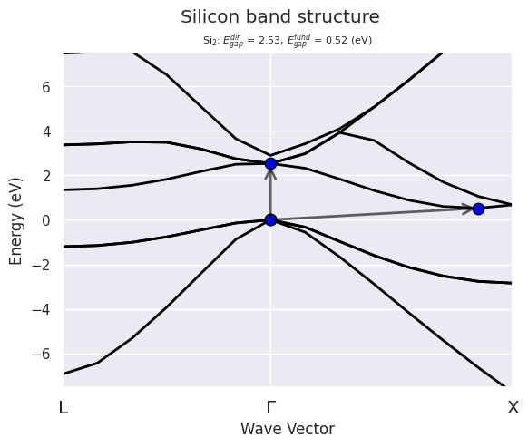
Direct gap:
Energy: 2.532 (eV)
Initial state: spin: 0, kpt: [+0.000, +0.000, +0.000], weight: 0.002, band: 3, eig: 5.598, occ: 2.000
Final state: spin: 0, kpt: [+0.000, +0.000, +0.000], weight: 0.002, band: 4, eig: 8.130, occ: 0.000
Fundamental gap:
Energy: 0.562 (eV)
Initial state: spin: 0, kpt: [+0.000, +0.000, +0.000], weight: 0.002, band: 3, eig: 5.598, occ: 2.000
Final state: spin: 0, kpt: [+0.375, +0.375, +0.000], weight: 0.012, band: 4, eig: 6.161, occ: 0.000
Bandwidth: 11.856 (eV)
Valence maximum located at kpt index 0:
spin: 0, kpt: [+0.000, +0.000, +0.000], weight: 0.002, band: 3, eig: 5.598, occ: 2.000
Conduction minimum located at kpt index 17:
spin: 0, kpt: [+0.375, +0.375, +0.000], weight: 0.012, band: 4, eig: 6.161, occ: 0.000
TIP: Use `--verbose` to print k-point coordinates with more digits
Important
In python we start to count from zero, thus the first band has index 0 and the first spin is 0 AbiPy uses the same convention so be very careful when specifying band, spin or k-point indices.
A GSR file produced by a self-consistent run, contains the values of the total energy, the forces, and the stress tensor at the end of the SCF cycle:
print("energy:", gsr.energy, "pressure:", gsr.pressure)
energy: -241.23647031321218 eV pressure: -5.211617575719521 GPa
To get a summary of the most important results:
print(gsr)
================================= File Info =================================
Name: si_scf_GSR.nc
Directory: /home/runner/work/abipy_book/abipy_book/abipy/abipy/data/refs/si_ebands
Size: 14.83 kB
Access Time: Thu Jan 15 12:16:05 2026
Modification Time: Thu Jan 15 12:15:09 2026
Change Time: Thu Jan 15 12:15:09 2026

================================= Structure =================================
Full Formula (Si2)
Reduced Formula: Si
abc   :   3.866975   3.866975   3.866975
angles:  60.000000  60.000000  60.000000
pbc   :       True       True       True
Sites (2)
  #  SP       a     b     c  cartesian_forces
---  ----  ----  ----  ----  -----------------------------------------------------------
  0  Si    0     0     0     [-5.89948307e-27 -1.93366149e-27  2.91016904e-27] eV ang^-1
  1  Si    0.25  0.25  0.25  [ 5.89948307e-27  1.93366149e-27 -2.91016904e-27] eV ang^-1
min |F_iat|: 6.856532001208972e-27 eV/Ang
max |F_iat|: 6.856532001208972e-27 eV/Ang
mean F_iat|: 6.856532001208972e-27 eV/Ang
std  |F_iat|: 0.0 eV/Ang
Forces are relaxed within high quality criterion: 0.0001 eV/Ang

Abinit Spacegroup: spgid: 227, num_spatial_symmetries: 48, has_timerev: True, symmorphic: True

Stress tensor (Cartesian coordinates in GPa):
[[5.21161758e+00 7.86452261e-11 0.00000000e+00]
 [7.86452261e-11 5.21161758e+00 0.00000000e+00]
 [0.00000000e+00 0.00000000e+00 5.21161758e+00]]

Pressure: -5.212 (GPa)
Energy: -241.23647031 (eV)

============================== Electronic Bands ==============================
Number of electrons: 8.0, Fermi level: 5.598 (eV)
nsppol: 1, nkpt: 29, mband: 8, nspinor: 1, nspden: 1
smearing scheme: none (occopt 1), tsmear_eV: 0.272, tsmear Kelvin: 3157.7
Direct gap:
    Energy: 2.532 (eV)
    Initial state: spin: 0, kpt: [+0.000, +0.000, +0.000], weight: 0.002, band: 3, eig: 5.598, occ: 2.000
    Final state:   spin: 0, kpt: [+0.000, +0.000, +0.000], weight: 0.002, band: 4, eig: 8.130, occ: 0.000
Fundamental gap:
    Energy: 0.562 (eV)
    Initial state: spin: 0, kpt: [+0.000, +0.000, +0.000], weight: 0.002, band: 3, eig: 5.598, occ: 2.000
    Final state:   spin: 0, kpt: [+0.375, +0.375, +0.000], weight: 0.012, band: 4, eig: 6.161, occ: 0.000
Bandwidth: 11.856 (eV)
Valence maximum located at kpt index 0:
    spin: 0, kpt: [+0.000, +0.000, +0.000], weight: 0.002, band: 3, eig: 5.598, occ: 2.000
Conduction minimum located at kpt index 17:
    spin: 0, kpt: [+0.375, +0.375, +0.000], weight: 0.012, band: 4, eig: 6.161, occ: 0.000

TIP: Use `--verbose` to print k-point coordinates with more digits
The different contributions to the total energy are stored in a dictionary:
print(gsr.energy_terms)
Term                  Value
e_localpsp            -68.62575673513619 eV
e_eigenvalues         4.453251818688362 eV
e_ewald               -226.94266726062642 eV
e_hartree             14.989583992483517 eV
e_corepsp             2.2624802653426976 eV
e_corepspdc           0.0 eV
e_kinetic             80.66035184380631 eV
e_nonlocalpsp         52.15353088289424 eV
e_entropy             0.0 eV
entropy               0.0 eV
e_xc                  -95.73399330197637 eV
e_xcdc                0.0 eV
e_paw                 0.0 eV
e_pawdc               0.0 eV
e_elecfield           0.0 eV
e_magfield            0.0 eV
e_fermie              5.598453325101502 eV
e_sicdc               0.0 eV
e_exactX              0.0 eV
h0                    0.0 eV
e_electronpositron    0.0 eV
edc_electronpositron  0.0 eV
e0_electronpositron   0.0 eV
e_monopole            0.0 eV
At this point, we don’t need this file anymore so we close it with:
gsr.close()
Warning
The gsr maintains a reference to the underlying netcdf file hence one should
call gsr.close() to release the resource when we don’t need it anymore.
Python will do it automatically if you use abiopen and the with context manager.
Note that we don’t always follow this rule inside the jupyter notebook to maintain the code readable but you should definitively close all your files, especially when writing code that may be running for hours or even more.
Plotting band structures#
Let’s open the GSR file produced by a NSCF calculation done on a high-symmetry k-path and extract the electronic band structure.
A warning is issued by pymatgen about the structure not being standard. Be aware that this might possibly affect the automatic labelling of the boundary k-points on the k-path. So, check carefully the k-point labels on the figures that are produced in such case. In the present case, the labelling is correct.
with abilab.abiopen(abidata.ref_file("si_nscf_GSR.nc")) as nscf_gsr:
    ebands_kpath = nscf_gsr.ebands
Now we can plot the band energies with matplotlib:
# The labels for the k-points are found in an internal database.
ebands_kpath.plot(with_gaps=True, title="Silicon band structure");
Alternatively, one can use the optional argument klabels to define the mapping
reduced_coordinates --> name of the k-point and pass it to the plot method
klabels = {
    (0.5, 0.0, 0.0): "L",
    (0.0, 0.0, 0.0): "$\Gamma$",
    (0.0, 0.5, 0.5): "X"
}

# ebands_kpath.plot(title="User-defined k-labels", band_range=(0, 5), klabels=klabels);
For the plotly version, use:
ebands_kpath.plotly(with_gaps=True, title="Silicon band structure with plotly");
abilab.abipanel()
gsr.get_panel()
Let’s have a look at our k-points by calling kpoints.plot()
ebands_kpath.kpoints.plotly();
and the crystalline structure with:
ebands_kpath.structure.plot();
Note
The same piece of code works if you replace the GSR.nc file with e.g. a WFK.nc file in netcdf format
(actually any netcdf file with an ebands object).
The main advantage of the GSR file is that it is lightweight (no wavefunctions).
DOS with the Gaussian technique#
Let’s use the eigenvalues and the k-point weights stored in gs_ebands to
compute the DOS with the Gaussian method.
The method is called without arguments so we use default values
for the broadening and the step of the linear mesh.
 with abilab.abiopen(abidata.ref_file("si_scf_GSR.nc")) as scf_gsr:
    ebands_kmesh = scf_gsr.ebands

edos = ebands_kmesh.get_edos()
print(edos)
  Cell In[16], line 1
    with abilab.abiopen(abidata.ref_file("si_scf_GSR.nc")) as scf_gsr:
    ^
IndentationError: unexpected indent
edos.plotly();
print("[ebands_kmesh] is_ibz:", ebands_kmesh.kpoints.is_ibz, "is_kpath:", ebands_kmesh.kpoints.is_path)
print("[ebands_kpath] is_ibz:", ebands_kpath.kpoints.is_ibz, "is_kpath:", ebands_kpath.kpoints.is_path)
Warning
The DOS requires a homogeneous \(k\)-sampling of the BZ. Abipy will raise an exception if you try to compute the DOS with a k-path.
To plot bands and DOS on the same figure:
ebands_kpath.plotly_with_edos(edos, with_gaps=True);
To plot the DOS and the integrated DOS (IDOS), use:
edos.plotly_dos_idos();
The gaussian broadening can significantly change the overall shape of the DOS. If accurate values are needed (e.g. the DOS at the Fermi level in metals), one should perform an accurate convergence study with respect to the k-point mesh. Here we show how compute the DOS with different values of the gaussian smearing for fixed k-point sampling and plot the results:
# Compute the DOS with the Gaussian method and different values of the broadening
widths = [0.1, 0.2, 0.3, 0.4]

edos_plotter = ebands_kmesh.compare_gauss_edos(widths, step=0.1)
To plot the results on the same figure, use:
edos_plotter.combiplot(title="e-DOS as function of the Gaussian broadening");
while gridplot generates a grid of subplots:
edos_plotter.gridplot();
Joint density of states#
This example shows how to plot the different contributions to the electronic joint density of states (JDOS) of Silicon. Select the valence and conduction bands to be included in the JDOS. Here we include valence bands from 0 to 3 and the first conduction band (4).
vrange = range(0,4)
crange = range(4,5)

# Plot data
ebands_kmesh.plot_ejdosvc(vrange, crange);
ebands_kpath.plot_transitions(omega_ev=3.0);
ebands_kmesh.plot_transitions(omega_ev=3.0);
Plotting the Fermi surface#
with abilab.abiopen(abidata.ref_file("mgb2_kmesh181818_FATBANDS.nc")) as fbnc_kmesh:
    mgb2_ebands = fbnc_kmesh.ebands

    # Build ebands in full BZ.
    mgb2_eb3d = mgb2_ebands.get_ebands3d()
There are three bands crossing the Fermi level of \(MgB_2\) (band 2, 3, 4):
mgb2_ebands.boxplot();
Let’s use matplotlib to plot the isosurfaces corresponding to the Fermi level (default):
# Warning: requires skimage package, rendering could be slow.
mgb2_eb3d.plot_isosurfaces();
#ebands_kpath.plot_scatter3d(band=3);
#ebands_kmesh.plot_scatter3d(band=3);
Analyzing multiple GSR files with robots#
TODO
Note
Robots can also be constructed from the command line with: abicomp.py gsr FILES