Theory#
This chapter presents the theoretical formalism behind the computation of the luminescence properties of point defects in solids. It starts with a section dedicated to the theory of luminescence, showing how Fermi’s golden rule is approximated to obtain a tractable way of computing the luminescence lineshape, following either an effective phonon mode model or a multi-phonon mode model. Then, the computational methodology used to obtain the parameters entering the lineshape equation is presented. Subtleties regarding the increase of the phonon supercell size thanks to the use of the forces instead of displacements are discussed. Finally, the IFCs embedding approach, that allows to compute the phonon modes of a defect system in large supercells, is presented.
From the Fermi’s Golden rule to the luminescence lineshape#
Following Fermi’s golden rule, the absolute luminescence intensity \(I(\hbar\omega)\) (number of photons per unit time per unit energy) associated to one emitting center with two states e and g, is expressed as a function of the photon energy \(\hbar\omega\) as
where \(n_D\) is the material refractive index, \(\boldsymbol{\mu_{eg}}=\langle\Psi_{e}|\boldsymbol{\mu}|\Psi_{g}\rangle\) is the total dipole matrix element. It is then assumed that the electronic part of the dipole matrix element between the excited and ground state depends weakly on the nuclear coordinates (Franck-Condon approximation). We also suppose that the nuclear motions can be expressed as a superposition of 3N harmonic normal modes of vibration \(\nu\), represented by normal coordinates \(Q_{\nu}\) and frequency \(\omega_{\nu}\), with N being the number of atoms in the cell considered. The total vibrational state \(\chi_{\boldsymbol{n}}\) is the product of 3N independent harmonic oscillator eigenfunctions \(\chi_{\boldsymbol{n_{\nu}}}\) with \(n_{\nu}\) the vibrational state of the \(\nu\)-th harmonic oscillator. We write the normalized luminescence intensity as
with C a normalization constant. In the case of the absolute intensity \(I(\hbar\omega)=C\omega^3A(\hbar\omega)\), \(C=\frac{n_D}{3 \pi \hbar \epsilon_0 c^3}|\boldsymbol{\mu}_{eg}^{el}|^2\) with \(\boldsymbol{\mu}_{eg}^{el}\) the purely electronic dipole moment (inversely proportional to the radiative lifetime of the emitting center). The emission lineshape function \( A(\hbar \omega)\), which dictates the shape of the spectrum, writes
In equation (26), \(\boldsymbol{n}\) denotes the set of 3N vibrational states {\(n_1\),\(n_2\),…,\(n_{3N}\)}, \(E_{ZPL}\) is the so-called zero-phonon line energy (purely electronic energy difference), \(E_{g/e,\boldsymbol{n/m}}=\sum{_\nu}n_{\nu}\hbar\omega_{g/e,\nu}\) is the vibrational energy of state \(\chi_{g/e,\boldsymbol{n/m}}\), and \(p_{_{\nu}}(T)\) is a Bose-Einsten thermal occupation factor.
The vibrational modes of the excited and ground states can be in principle different, making equation (26) computationally very expensive because of the highly multidimensional integrals to be evaluated (Franck-condon overlaps). Some approximations should be made. We assume first that the vibrational modes in the excited electronic state are identical to those in the ground state. We also assume that we work at T=0 K, to alleviate the equations (\(p_{m_{\nu}}(T=0)\) = 0 if \(m_{\nu}\) a vibrational state of the electronic excited state is different from 0). Considering temperature dependent luminescence spectrum will be presented later.
Effective phonon mode model#
The simplest model to start with is built when considering that the 3N phonon modes of the system can be reduced to a single effective phonon mode. Suppose that a single effective mode couples to the electronic transition, the Franck-Condon overlaps will reduce to \(|\langle\chi_{e,0}|\chi_{g,n}\rangle|^2\). In the harmonic approximation, the vibrational eigenfunctions \(\chi\) are expressed with Hermite polynomials and their overlaps can be computed analytically :
with \(S\) the Huang-Rhys factor, a dimensionless constant giving the mean number of effective phonons of frequency \(\Omega\) involved in the electronic transition,
and \(\Delta Q\) the offset between the harmonic potential energy surface of the ground and excited state. In practice, such offset is computed as a total mass weighted atomic displacements induced by the electronic transition:
where \(i\) labels the cartesian axes, \(\kappa\) the atoms, \(m_{\kappa}\) atomic masses, \(R_{e;\kappa i}\) and \(R_{g;\kappa i}\) are respectively atomic positions in the excited and the ground states.
This allows to simplify equation (26) to
A schematic figure of such model is presented on figure Fig. 1 for a single mode \(\nu\).
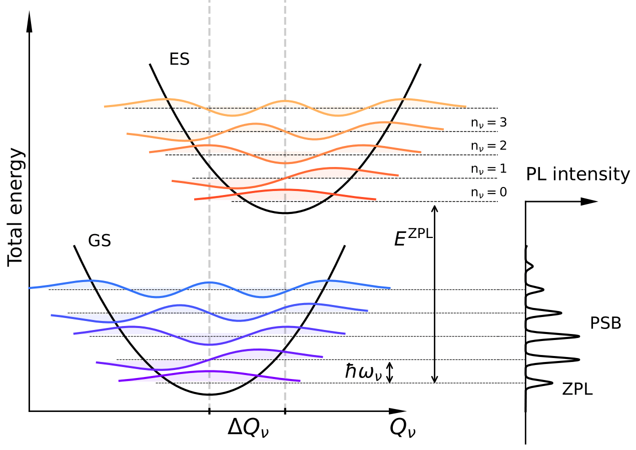
Fig. 1 Schematic representation of the origin of photoluminescence (PL) spectra. On the left, ground state (GS) and excited state (ES) energy curves are projected along phonon normal coordinate \(Q_{\nu}\) (here only for one mode) and are approximated by harmonic functions with the same frequency \(\omega_{\nu}\). Vibrational energy levels and corresponding eigenfunctions are shown as horizontal lines and colored areas. GS and ES are displaced by \(\Delta Q_{\nu}\), the mass-weighted displacement between the minimum of the GS and the ES curves. On the right, the PL spectrum is formed. The zero-phonon line (ZPL) comes from the transition between the first vibrational level of the ES to the first vibrational level of the GS. Other transitions give the phonon sideband (PSB). The intensity of each peak is computed with the overlap between corresponding eigenfunctions.#
Multi phonon mode model and generating function#
We now consider the 3N vibrational modes. Quantities of the above section are now computed “per phonon mode”. The \(\Delta Q_{\nu}\) (mass-weighted atomic displacement projected along phonon mode \(\nu\))
are used to compute the partial Huang-Rhys factor \(S_\nu=\frac{\omega_\nu\Delta Q_\nu^2}{2\hbar}\). \(e_{\nu,\kappa\alpha}\) are the phonon eigenvectors. These define the Huang-Rhys spectral function:
When dealing with 3N phonons, a direct evaluation of equation (26) is impractical. Instead, the so-called generating function approach is used. The lineshape function \(A(\hbar\omega)\) is evaluated as the Fourier transform of the generating function \(G(t)\)
with
where \(S(t)=\sum_\nu S_\nu e^{i\omega_\nu t}\) is the Fourier transform of the Huang-Rhys spectral function. \(\gamma\) is a constant homogeneous Lorentzian broadening associated to each vibronic transition.
While working in the time domain, the effect of temperature (transitions involving initial vibrational states \(n_{\nu} \ne 0\), weighted by Bose-Einstein occupation) can be included straightforwardly by rewriting the generating function
with \(C(t,T)=\sum_\nu\overline{n}_\nu(T)S_\nu e^{i\omega_\nu t}\) the Fourier transform of the temperature weighted Huang-Rhys spectral function, and \(\overline{n}_\nu(T)\) the average occupation number of \(\nu\)-th phonon mode:
One can connect the multi-phonon modes methodology to the simpler effective phonon mode model presented in the previous section. The total normal coordinate change \(\Delta Q\), due to the orthonormality of the phonon eigenvectors is linked through the partial \(\Delta Q_{\nu}\) through:
and allows one to define the weight by which a mode contributes to the total atomic relaxation:
It is then possible to define an effective frequency as
and the total Huang-Rhys factor as:
Semi-classical approach#
Within a semi-classical formulation [Henderson and Imbusch, 2006], one can find formulas for the full width a half maximum of the emission shape:
where \(S_{\mathrm{em}}\) and \(S_{\mathrm{abs}}\) are the Huang-Rhys factors associated to the emission and absorption processes respectively, and \(\Omega_{\mathrm{g}}\) is the effective frequency of the ground state.
Averaging the Bose-Einstein occupations of the initial vibrational states allows one to compute the temperature dependent FWHM:
Computational methodology#
From the above approximations, we see that the photo-luminescent lineshape of a point defect in a solid is uniquely defined by the Huang-Rhys spectral function \(S(\hbar\omega)\) and the zero-phonon line. In order to compute it from first-principles, we need to obtain:
The zero-phonon line energy \(E_{ZPL}\), which is the total energy difference between the electronic excited and ground states of the system.
The atomic relaxation associated to the change in electronic state, obtained as the difference between the relaxed atomic positions of the excited state and relaxed atomic positions of the ground state.
The vibrational modes of the system. Note that in the case of the effective phonon model, this is not required since the effective mode is obtained from the atomic relaxation.
One way to obtain the first two parameters is to use DFT following the \(\Delta SCF\) constrained occupation method. The vibrational modes can be obtained with finite difference or DFPT, or by using the embedding methodology presented in latter in this chapter.
\(\Delta\)SCF constrained occupation method#
This method refers to the use of DFT with non-Aufbau electronic occupations to mimick the electron-hole interaction. Transition energies are computed by taking the differences between total DFT energies with different occupations. Note that the excited state occupations are specific to the system under study. In the case of Eu\(^{2+}\), one of the seven 4f electron of the spin-up channel is promoted to the next spin-up 5d energy state, as shown in Fig. 2. This figure also illustrates the connection with the configuration coordinate model.
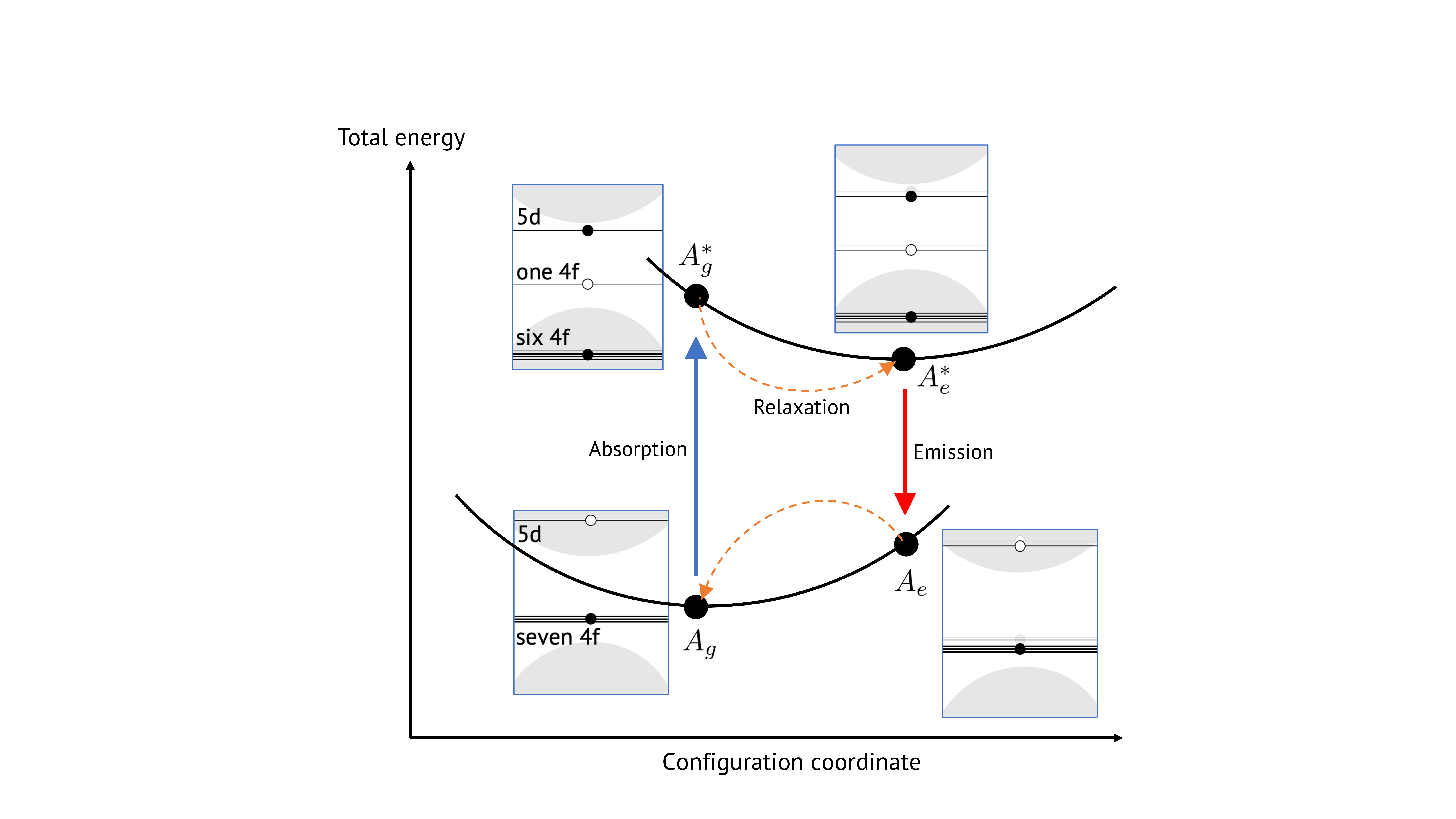
Fig. 2 Schematic representation of the constrained occupation \(\Delta\)SCF method, as used in this work for simulating the luminescent properties of Eu\(^{2+}\) phosphor.#
The procedure is as follows:
Start with a relaxed ground state (labeled \(A_g\)) with energy \(E_{g}\).
Promote an electron to obtain the excited state configuration (\(A_g^*\), energy \(E_{g}^{*}\)). The difference in energy with the \(A_g\) state provides an estimate of the semi-classical absorption energy:
(43)#\[ E_{\mathrm{abs}} = E_{g}^{*} - E_{g} \]After structural relaxation in the excited state, obtain the relaxed excited state (\(A_e^*\), energy \(E_e^*\)), which allows computation of the zero-phonon line (ZPL) energy:
(44)#\[ E_{\mathrm{ZPL}} = E_e^* - E_g \]The Franck-Condon relaxation energy of the excited state is:
(45)#\[ E_{\mathrm{FC,e}} = E_{g}^{*} - E_{e}^{*} \]De-promoting the electron with the relaxed atomic positions of the excited state yields the ground state with excited geometry (\(A_e\), energy \(E_e\)). The emission energy is:
(46)#\[ E_{\mathrm{em}} = E_e^* - E_e \]The Franck-Condon relaxation energy of the ground state is:
(47)#\[ E_{\mathrm{FC,g}} = E_{e} - E_{g} \]
Assuming harmonicity, the effective frequencies of the ground or excited states can be extracted as
where \(\Delta Q\) is the mass-weighted atomic displacement between the ground and excited states, as defined in equation (29). The corresponding Huang-Rhys factors can be obtained from (28).
Forces vs Displacements, increase of supercell size#
For a given phonon mode \(\nu\), the corresponding partial Huang-Rhys factor \(S_{\nu}=\frac{\omega_{\nu}\Delta Q_{\nu}^2}{2\hbar}\) is computed thanks to the mass-weighted displacement between ground and excited states projected on this phonon mode:
where \(\kappa\) labels the atoms and \(\alpha\) the cartesian direction. Under the harmonic approximation,
with the interatomic force constants (IFCs) \(C_{\kappa,\kappa'}=\frac{\Delta F_{\kappa'}}{\Delta R_{\kappa}}\), Eq. (49) rewrites:
The use of Eq.(51) allows increasing the supercell size and hence minimize finite-size effects.
Indeed, the forces decay faster to zero compared to the displacements with respect to the distance from the defect as illustrated in see Fig. 3, panel a-b.
We assume that the forces computed within the small red supercell (here 288 atoms), see Fig. 3, panel c , are already converged and without finite-size effect because of this rapid decay, and that the forces outside this red supercell are essentially zero.
This means that we can use the forces computed in this red supercell, and deduce the displacements at much larger distance in the blue supercell via the IFCs computed within this large blue supercell.
This subtle point is actually directly included when using Eq.(51) in the blue supercell. This also means that the IFCs/phonons modes should be computed in the same blue supercell. This is discussed in the next section.
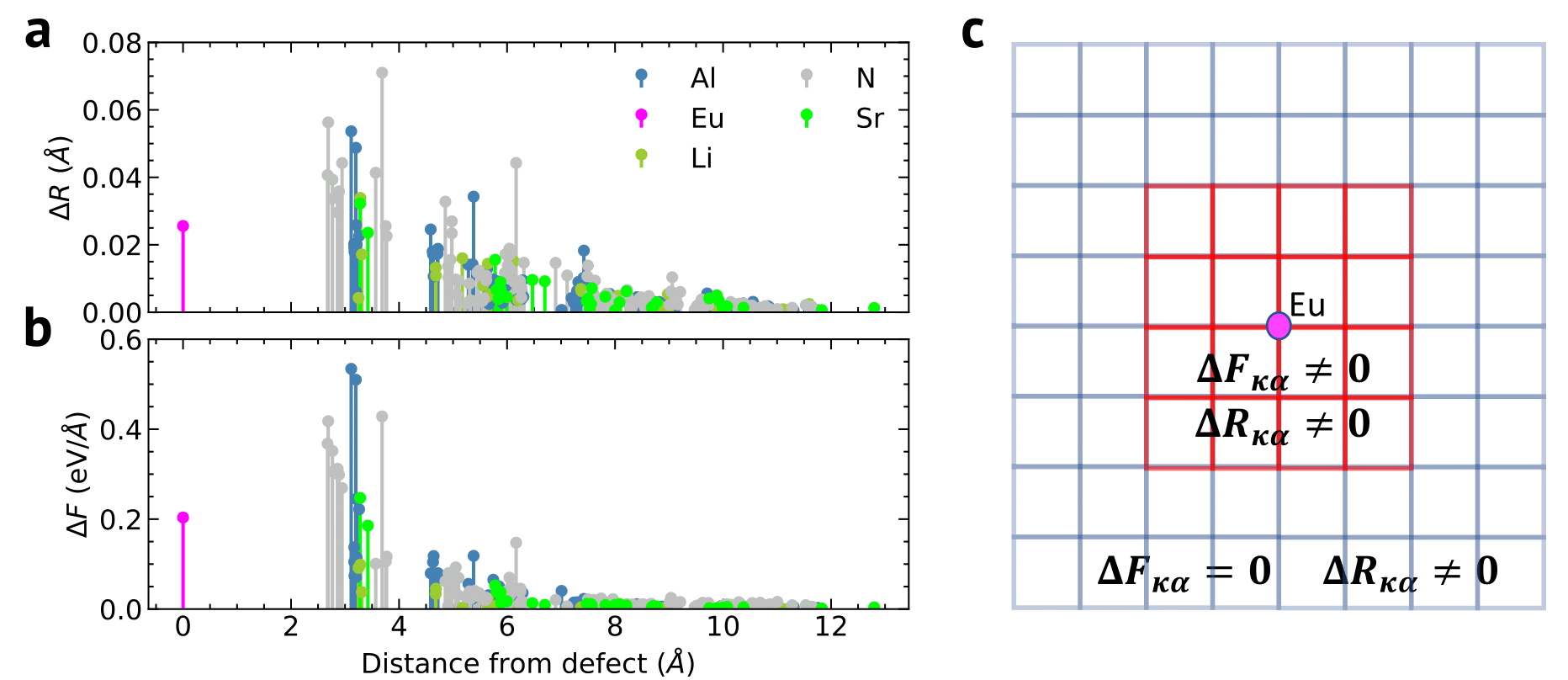
Fig. 3 (a) Norm of the displacement induced by an electronic transition as a function of the distance from the defect atom (Eu). (b) Norm of the forces in the ground state at the excited state equilibrium atomic positions. The decay of forces (b) is much faster than the decay of displacements (a). © Cartoon of a small red supercell containing substitutional defect where the forces are the ones computed with DFT. Outside this red supercell, the forces are set to zero because of their short-range decay while the displacements are non-zero and are computed with the IFCs computed in this large blue supercell.#
IFCs embedding#
In the computation of the partial Huang-Rhys factors, one would like to obtain the phonons in very large supercells at wave vector \(\mathbf{q}\rightarrow(0,0,0)\) (\(\Gamma\) point), so that the coupling with long-wavelength phonons is correctly captured. One would also like to include the coupling with (localized) phonons modes introduced by the defect. A direct approach, either with DFPT or finite difference, is not computationally attractive. Indeed, DFPT is best used for small pristine primitive cells at dense \(\mathbf{q}\)-mesh (which corresponds to large pristine supercells after a folding procedure), while finite difference, for which the introduction of defect does not cause problem, remains costly for large supercells. One way to include both the defect effect (local modes) while converging long-wavelength phonons is to employ the IFCs embedding approach [Alkauskas et al., 2014, Jin et al., 2021].
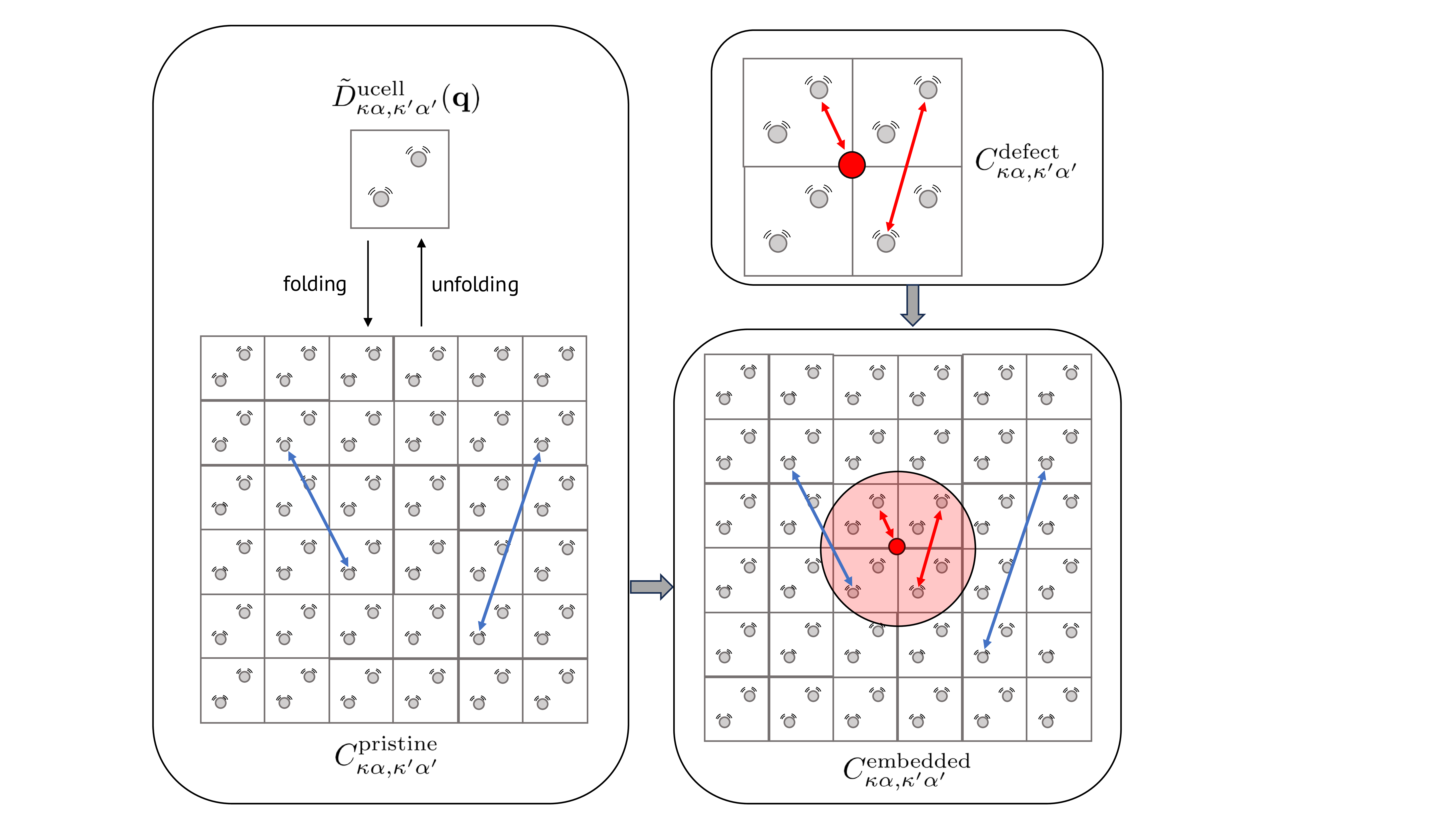
Fig. 4 Schematic view of the interatomic force constants (IFC) embedding approach to obtain defect phonons in large supercells. Each arrow represents an IFC between a pair of two atoms. See text for details.#
The procedure, illustrated in figure Fig. 4, is as follows:
First, the real-space interatomic force constants (IFCs) of the defect system, denoted as \(C_{\kappa\alpha,\kappa’\alpha}^{\mathrm{defect}}\), are computed within a relatively small supercell (typically with a few hundred atoms). This is often done using a finite difference approach on the supercell at the \(\Gamma\) point, though Density Functional Perturbation Theory (DFPT) could also be employed if the memory requirements are manageable and/or if the level of theory required to describe the defect (e.g., DFT+U) is supported by the DFPT code.
Second, the IFCs of the pristine system, \(C_{\kappa\alpha,\kappa’\alpha}^{\mathrm{pristine}}\), are obtained within a much larger supercell (typically with a few thousand atoms). A practical approach is to use DFPT on the unit cell to calculate the dynamical matrix on a \(\mathbf{q}\)-mesh, potentially followed by Fourier interpolation to obtain the matrix on a denser [\(N_x,N_y,N_z\)] \(\mathbf{q}\)-mesh. The information in the dynamical matrix, computed on a unit cell for a dense [\(N_x,N_y,N_z\)] \(\mathbf{q}\)-mesh, is equivalent to that in a dynamical matrix for a [\(N_x,N_y,N_z\)] supercell at \(\mathbf{q} = [0,0,0]\) (the \(\Gamma\) point). Mapping a \(\mathbf{q}\)-mesh to \(\mathbf{q} = [0,0,0]\) is referred to a folding procedure, and yields the pristine IFCs \(C_{\kappa\alpha,\kappa’\alpha}^{\mathrm{pristine}}\).
Third, an embedded IFC matrix \(C_{\kappa\alpha,\kappa’\alpha}^{\mathrm{emb}}\) is constructed using the following rules: If both atoms \(\kappa\) and \(\kappa’\) are within a sphere centered around the defect, with a cut-off radius \(R_c\), then \(C_{\kappa\alpha,\kappa’\alpha}^{\mathrm{emb}}\) is set to \(C_{\kappa\alpha,\kappa’\alpha}^{\mathrm{defect}}\). For all other atomic pairs, the embedded IFC is set to the pristine value: \(C_{\kappa\alpha,\kappa’\alpha}^{\mathrm{emb}} = C_{\kappa\alpha,\kappa’\alpha}^{\mathrm{pristine}}\). The cut-off radius \(R_c\) is typically determined by the size of the initial supercell used to compute the defect IFCs. Additionally, one could use a second cut-off radii \(R_b\). If two atoms are not within a sphere of radii \(R_b\), the IFC is set to zero. The use of this second cut-off has been used in some studies [Jin et al., 2021, Razinkovas et al., 2021] in order to obtain large sparse matrices, for which dedicated techniques allows faster diagonalization, see for instance reference [Razinkovas et al., 2021]. In this work, we do not use this second cut-off.
Overall, the whole procedure can break the acoustic sum rule
To correct for this, we follow the same approach that in [Jin et al., 2021, Razinkovas et al., 2021]:
For the treatment of the Born effective charges (BECs), if the BEC of the substituted atom was computed in the defect phonon calculation, it is replaced by the BEC of the dopant atom. If not, one can choose to use the most common oxidation state of the dopant atom as its new BEC. The same approach applies to interstitials, but in this case, the dopant atom and its corresponding BEC are simply added. For vacancies, the atom and its BEC are removed.
Diagonalizing this embedded IFCs provides the phonon modes of a defectuous [\(N_x,N_y,N_z\)] supercell, where the defect effect on the IFCs was included through the embedding procedure.
The localization of the phonon modes can be characterized by computing the inverse participation ratio (IPR) defined as [Alkauskas et al., 2014, Jin et al., 2021]
where \(\mathbf{e}_{\nu,\kappa}\) is the eigenvector of the phonon mode \(\nu\) associated to atom \(\kappa\). The IPR is a measure of the localization of the phonon mode \(\nu\) and is normalized to the number of atoms in the supercell \(N\). The IPR can be interpreted as a measure of the number of atoms that participate in a given phonon mode, which indicates, roughly speaking, the number of atoms that participate to a phonon mode \(\nu\). For example, \(\mathrm{IPR}_{\nu}=1\) means that only one atom vibrates and therefore the phonon mode is maximally localized, while \(\mathrm{IPR}_{\nu}=N\) means that N atoms vibrates in the supercell with the same amplitude.
The localization ratio \(\beta_{\nu}\) is defined by taking the ratio of the total number of atoms in the supercell \(N\) and the \(\rm{IPR}\), \(\beta_{\nu} =N/\mathrm{IPR}_{\nu}\) where \(\beta_{\nu} \approx 1\) represents a bulk-like delocalized mode while \(\beta_{\nu} \gg 1\) corresponds to a quasi-local or local mode.
References#
Brian Henderson and G Frank Imbusch. Optical spectroscopy of inorganic solids. Volume 44. Oxford University Press, 2006.
Audrius Alkauskas, Bob B Buckley, David D Awschalom, and Chris G Van de Walle. First-principles theory of the luminescence lineshape for the triplet transition in diamond NV centres. New J. Phys., 16(7):073026, 2014.
Yu Jin, Marco Govoni, Gary Wolfowicz, Sean E Sullivan, F Joseph Heremans, David D Awschalom, and Giulia Galli. Photoluminescence spectra of point defects in semiconductors: validation of first-principles calculations. Physical Review Materials, 5(8):084603, 2021.
Lukas Razinkovas, Marcus W Doherty, Neil B Manson, Chris G Van de Walle, and Audrius Alkauskas. Vibrational and vibronic structure of isolated point defects: the nitrogen-vacancy center in diamond. Physical Review B, 104(4):045303, 2021.
Julien Bouquiaux, Samuel Poncé, Yongchao Jia, Anna Miglio, Masayoshi Mikami, and Xavier Gonze. Importance of long-range channel sr displacements for the narrow emission in sr [li2al2o2n2]: eu2+ phosphor. Advanced Optical Materials, 9(20):2100649, 2021.
Julien Bouquiaux, Samuel Poncé, Yongchao Jia, Anna Miglio, Masayoshi Mikami, and Xavier Gonze. A first-principles explanation of the luminescent line shape of srlial3n4: eu2+ phosphor for light-emitting diode applications. Chemistry of Materials, 35(14):5353–5361, 2023.