Phonons and Born effective charges

This lesson discusses how to compute phonon band structures, DOS and Born effective charges with Abinit and AbiPy. The discussion closely follows the second lesson on DFPT available on the Abinit website. More specifically, we discuss how to:

• Perform a convergence study of the phonon frequencies at \(\Gamma\) as a function of ecut

• Compute the full phonon band structure of AlAs, including the LO-TO splitting

• Obtain thermodynamic properties within the harmonic approximation

We assume that you have read the references mentioned in the first Abinit lesson on DFPT. You may find additional material related to the present section in the following references:

• Dynamical matrices, Born effective charges, dielectric permittivity tensors, and interatomic force constants from density-functional perturbation theory

• Phonons and related crystal properties from density-functional perturbation theory

If you are already familiar with Python, and AbiPy and Abinit are already installed and configured, you may want to use the command-line interface directly. See the README.md file in the directory of this lesson, which explains how to analyze the data from the shell using IPython and matplotlib.

Note

AbiPy provides two different APIs to produce figures, with either matplotlib or plotly. In this tutorial, we use the plotly API as much as possible, although it should be noted that not all the plotting methods have been ported to plotly yet.

AbiPy uses a relatively simple rule to differentiate between the two plotting libraries: if an object provides an obj.plot method producing a matplotlib plot, the corresponding native plotly version (if available) is named obj.plotly. Note that plotly requires a web browser, hence the matplotlib version is still valuable if you need to visualize results on machines on which only an X server is available.

In AbiPy versions greater than 0.9, you can try to convert the matplotlib figures produced by plot methods into Plotly figures using the optional argument plotly=True, although the result is not always guaranteed.

Phonon frequencies at \(\Gamma\) as function of ecut

Before starting, we need to import the Python modules and the functions we will need in the notebook:

import numpy as np
import warnings

warnings.filterwarnings("ignore") # to get rid of deprecation warnings

from abipy import abilab
abilab.enable_notebook() # This line tells AbiPy we are running inside a notebook
import abipy.flowtk as flowtk

# This line configures matplotlib to show figures embedded in the notebook.
# Replace `inline` with `notebook` in classic notebook
%matplotlib inline

# Option available in jupyterlab. See https://github.com/matplotlib/jupyter-matplotlib
#%matplotlib widget

and a useful function from the lesson_dfpt module that will be used to generate our DFPT flows:

from lesson_dfpt import make_scf_input
abilab.print_source(make_scf_input)

def make_scf_input(ecut=2, ngkpt=(4, 4, 4)):
    """
    This function constructs an `AbinitInput` to perform a GS-SCF calculation in crystalline AlAs.

    Args:
        ecut: cutoff energy in Ha.
        ngkpt: 3 integers specifying the k-mesh for the electrons.

    Return:
        `AbinitInput` object
    """
    # Initialize the AlAs structure from an internal database. Use the pseudos shipped with AbiPy.
    gs_inp = abilab.AbinitInput(structure=abidata.structure_from_ucell("AlAs"),
                                pseudos=abidata.pseudos("13al.981214.fhi", "33as.pspnc"))

    # Set the value of the Abinit variables needed for GS runs.
    gs_inp.set_vars(
        nband=4,
        ecut=ecut,
        ngkpt=ngkpt,
        nshiftk=4,
        shiftk=[0.0, 0.0, 0.5,   # This gives the usual fcc Monkhorst-Pack grid
                0.0, 0.5, 0.0,
                0.5, 0.0, 0.0,
                0.5, 0.5, 0.5],
        ixc=1,
        nstep=25,
        diemac=9.0,
        tolvrs=1.0e-10,
        #iomode=3,
    )

    return gs_inp

The function makes some assumptions about important parameters such as the crystalline structure and the pseudos. This is done on purpose, to keep the code as simple as possible. It should not be difficult to generalize the implementation to other cases. Let’s start playing with our new function:

scf_input = make_scf_input()
scf_input

##############################################
#### SECTION: basic
##############################################
nband 4
ecut 2
ngkpt 4 4 4
nshiftk 4
shiftk
0.0 0.0 0.5
0.0 0.5 0.0
0.5 0.0 0.0
0.5 0.5 0.5
ixc 1
nstep 25
tolvrs 1e-10
##############################################
#### SECTION: files
##############################################
indata_prefix indata/in
tmpdata_prefix tmpdata/tmp
outdata_prefix outdata/out
pp_dirpath /home/runner/work/abipy_book/abipy_book/abipy/abipy/data/pseudos
pseudos 13al.981214.fhi 33as.pspnc
##############################################
#### SECTION: gstate
##############################################
diemac 9.0
##############################################
#### STRUCTURE
##############################################
natom 2
ntypat 2
typat 1 2
znucl 13 33
xred
0.0000000000 0.0000000000 0.0000000000
0.2500000000 0.2500000000 0.2500000000
acell 1.0 1.0 1.0
rprim
0.0000000000 5.3050000000 5.3050000000
5.3050000000 0.0000000000 5.3050000000
5.3050000000 5.3050000000 0.0000000000

print(scf_input.structure)

Full Formula (Al1 As1)
Reduced Formula: AlAs
abc   :   3.970101   3.970101   3.970101
angles:  60.000000  60.000000  60.000000
pbc   :       True       True       True
Sites (2)
  #  SP       a     b     c
---  ----  ----  ----  ----
  0  Al    0     0     0
  1  As    0.25  0.25  0.25

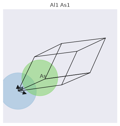
scf_input.structure.plot();

We are using the same pseudopotentials as in the official tutorial. Note that the XC functional is LDA in both pseudos, but with different parametrizations. This is why we specify ixc in the input file. This is not needed if you are using pseudos generated with the same ixc.

for pseudo in scf_input.pseudos:
    print(pseudo, "\n")

<NcAbinitPseudo: 13al.981214.fhi>
  summary: Aluminum, fhi98PP : Hamann-type, LDA CA PerdewWang, l=2 local
  number of valence electrons: 3.0
  maximum angular momentum: d
  angular momentum for local part: d
  XC correlation: PW
  supports spin-orbit: False
  radius for non-linear core correction: 0.0
  hint for low accuracy: ecut: 0.0, pawecutdg: 0.0
  hint for normal accuracy: ecut: 0.0, pawecutdg: 0.0
  hint for high accuracy: ecut: 0.0, pawecutdg: 0.0 

<NcAbinitPseudo: 33as.pspnc>
  summary: Troullier-Martins psp for element  As        Thu Oct 27 17:37:14 EDT 1994
  number of valence electrons: 5.0
  maximum angular momentum: p
  angular momentum for local part: p
  XC correlation: LDA_XC_TETER93
  supports spin-orbit: False
  radius for non-linear core correction: 2.0573171556401
  hint for low accuracy: ecut: 0.0, pawecutdg: 0.0
  hint for normal accuracy: ecut: 0.0, pawecutdg: 0.0
  hint for high accuracy: ecut: 0.0, pawecutdg: 0.0 

As you can see, we essentially have a standard input for a GS calculation. This object will be the building block of our DFPT calculation with AbiPy.

If this is not your first time using the DFPT part of Abinit, you already know that phonon calculations require an initial GS run to produce the WFK file, followed by a DFPT run that reads the WFK file and solves the Sternheimer equations for \(N_{\text{irred}}(q)\) atomic perturbations, where \(N_{\text{irred}}\) is the number of independent atomic displacements (assuming \(q\) belongs to the \(k\)-mesh).

If you try to do a convergence study with respect to ecut without multi-datasets, you will likely start from an initial GS input file with a given value of ecut, use it as a template to generate the DFPT input files, create symbolic links to the WFK file produced in the first GS step, and then instruct Abinit to read this file with irdwfk. Once you have a set of input files that work for a particular ecut, you can simply replicate the set of directories and files, and use a script to change the value of ecut in the input files. Then, of course, you have to run the calculations manually, collect the results and produce nice plots to understand what is happening.

This approach is obviously boring and error-prone for a human being, but it is easy to implement in an algorithm, and machines do not complain if they have a lot of repetitive work to do! There are also several technical advantages in using this task-based approach vs multi-datasets, but we will discuss this point in more detail later.

If the machine could speak, it would tell you: give me an object that represents an input for GS calculations, give me the list of \(q\)-points you want to compute as well as the parameters that must be changed in the initial input, and I will generate a Flow for DFPT calculations. This logic appears so frequently that we decided to encapsulate it in the flowtk.phonon_conv_flow factory function:

from lesson_dfpt import build_flow_alas_ecut_conv
abilab.print_source(build_flow_alas_ecut_conv)

def build_flow_alas_ecut_conv(options):
    """
    Build and return Flow for convergence study of phonon frequencies at Gamma as function of ecut.
    """
    scf_input = make_scf_input()
    return flowtk.phonon_conv_flow("flow_alas_ecut_conv", scf_input, qpoints=(0, 0, 0),
                                   params=["ecut", [4, 6, 8]])

Let’s call the function to build our flow:

flow = build_flow_alas_ecut_conv(options=None)

flow.show_info()

<Flow, node_id=131, workdir=flow_alas_ecut_conv>
Number of works: 6, total number of tasks: 9
Number of tasks with a given class:

Task Class      Number
------------  --------
ScfTask              3
PhononTask           6

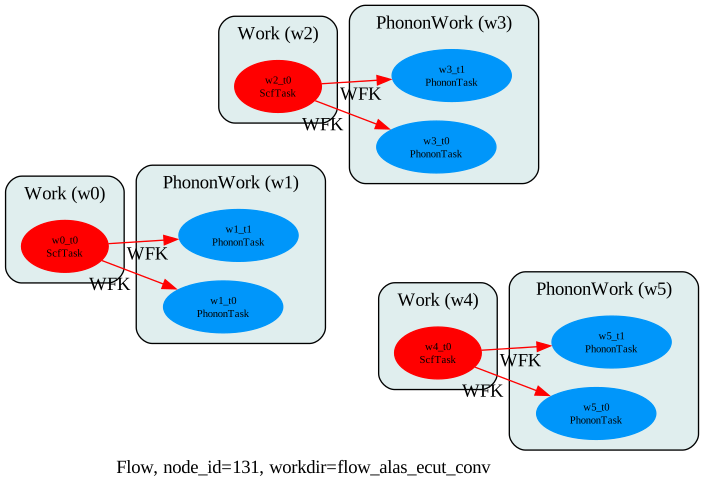
and call the get_graphviz method to visualize the connection among the Tasks:

flow.get_graphviz()

# matplotlib version based on networkx
#flow.plot_networkx(with_edge_labels=True);

The flow contains three independent groups of tasks, one for each value of ecut specified in params.

for work in flow:
    for task in work:
        print(task.pos_str, "uses ecut:", task.input["ecut"])

w0_t0 uses ecut: 4
w1_t0 uses ecut: 4
w1_t1 uses ecut: 4
w2_t0 uses ecut: 6
w3_t0 uses ecut: 6
w3_t1 uses ecut: 6
w4_t0 uses ecut: 8
w5_t0 uses ecut: 8
w5_t1 uses ecut: 8

flow.get_vars_dataframe("ecut")

	ecut	class
w0_t0	4	ScfTask
w1_t0	4	PhononTask
w1_t1	4	PhononTask
w2_t0	6	ScfTask
w3_t0	6	PhononTask
w3_t1	6	PhononTask
w4_t0	8	ScfTask
w5_t0	8	PhononTask
w5_t1	8	PhononTask

Each group represents a Work and consists of one ScfTask (red circle) that solves the KS equations self-consistently, producing a WFK file that is used by the two children (PhononTasks, blue circles) to compute the first-order change of the wavefunctions due to one of the irreducible atomic perturbations.

Note that phonon_conv_flow invokes Abinit under the hood to get the list of irreducible perturbations and uses this information to build the flow. This explains why we have two PhononTasks per \(q\)-point instead of one per phonon mode (\(3 N_{atom}=6\) in total).

Perhaps a table with the values of the input variables associated with the DFPT perturbations will help. None means that the variable is not defined in that particular input.

flow.get_vars_dataframe("rfphon", "rfatpol", "rfdir", "qpt", "kptopt")

	rfphon	rfatpol	rfdir	qpt	kptopt	class
w0_t0	None	None	None	None	None	ScfTask
w1_t0	1	[1, 1]	[1, 0, 0]	[0.0, 0.0, 0.0]	2	PhononTask
w1_t1	1	[2, 2]	[1, 0, 0]	[0.0, 0.0, 0.0]	2	PhononTask
w2_t0	None	None	None	None	None	ScfTask
w3_t0	1	[1, 1]	[1, 0, 0]	[0.0, 0.0, 0.0]	2	PhononTask
w3_t1	1	[2, 2]	[1, 0, 0]	[0.0, 0.0, 0.0]	2	PhononTask
w4_t0	None	None	None	None	None	ScfTask
w5_t0	1	[1, 1]	[1, 0, 0]	[0.0, 0.0, 0.0]	2	PhononTask
w5_t1	1	[2, 2]	[1, 0, 0]	[0.0, 0.0, 0.0]	2	PhononTask

If the meaning of these variables is not clear, you can consult the Abinit documentation, e.g. the documentation of the rfatpol input variable, or access the documentation directly from Python with:

abilab.docvar("rfatpol")

Default value:

[1, '[[natom]]']

Description:

Control the range of atoms for which displacements will be considered in phonon calculations (atomic polarizations). These values are only relevant to phonon response function calculations. May take values from 1 to natom, with rfatpol(1)<=rfatpol(2). The atoms to be moved will be defined by the do-loop variable iatpol:

• do iatpol=rfatpol(1),rfatpol(2)

For the calculation of a full dynamical matrix, use rfatpol(1)=1 and rfatpol(2)=natom, together with rfdir 1 1 1, both being the default values. For selected elements of the dynamical matrix, use different values of rfatpol and/or rfdir. The name 'iatpol' is used for the part of the internal variable ipert when it runs from 1 to natom. The internal variable ipert can also assume values larger than natom, denoting perturbations of electric field or stress type (see the DFPT help file).

As a side technical information, the value rfatpol(1)=-1 is admitted, and transformed immediately to rfatpol(1)=1, while rfatpol(2)=-1 is transformed to rfatpol(2)=natom, while the default input values are actually rfatpol=-1 .

Note

For your convenience, the links to the documentation of the different variables are listed below:

• qpt

• rfphon

• rfatpol

• rfdir

• kptopt

Now we can generate the flow_alas_ecut_conv directory with the input files by executing the lesson_dfpt.py script. Then use the abirun.py script to launch the entire calculation with:

abirun.py flow_alas_ecut_conv scheduler

You will see that all the PhononTasks are executed in parallel on your machine.

Warning

Please make sure that AbiPy is properly configured by running abicheck.py --with-flow.

If you prefer to skip this part, you can jump to the next section, which presents the post-processing of the results. Note that the output files are already available in the repository, so you can also try the AbiPy post-processing tools without having to run the flow.

Convergence study at \(\Gamma\)

There are several output files located inside the outdata directories:

!find flow_alas_ecut_conv/ -name "*_DDB"

flow_alas_ecut_conv/w5/outdata/out_DDB
flow_alas_ecut_conv/w1/outdata/out_DDB
flow_alas_ecut_conv/w4/t0/outdata/out_DDB
flow_alas_ecut_conv/w0/t0/outdata/out_DDB
flow_alas_ecut_conv/w2/t0/outdata/out_DDB
flow_alas_ecut_conv/w3/outdata/out_DDB

Remember that our goal is to analyze the convergence of the phonon frequencies at \(\Gamma\) as a function of ecut. So we are mainly interested in the DDB files located in the outdata directories of the PhononWorks (w0/outdata, w1/outdata, w2/outdata). These DDB files contain all the information needed to reconstruct the dynamical matrix at \(\Gamma\) and to compute the phonon frequencies (AbiPy calls mrgddb to merge the DDB files once all the perturbations in the PhononWork have been computed).

The code below tells our robot that we would like to analyze all the DDB files located in the output directories of the works:

robot = abilab.DdbRobot.from_dir_glob("./flow_alas_ecut_conv/w*/outdata/")
robot

0. flow_alas_ecut_conv/w5/outdata/out_DDB
1. flow_alas_ecut_conv/w1/outdata/out_DDB
2. flow_alas_ecut_conv/w3/outdata/out_DDB

For more examples on the use of DDB files and robots, see the DDB notebook. Now we ask the robot to call anaddb to compute the phonon frequencies at \(\Gamma\) for all the DDBs. The results are returned in a PhqData object, whose ph_df attribute is a pandas DataFrame:

ph_data = robot.get_phdata_at_qpoint((0, 0, 0))
data_gamma = ph_data.ph_df

Calculation completed. Anaddb results available in: /tmp/tmpeskrrv_i

Calculation completed. Anaddb results available in: /tmp/tmpztrnrebs

Calculation completed. Anaddb results available in: /tmp/tmp0553ad6t

The DataFrame is a dict-like object whose keys are the names of the columns in the table:

print(data_gamma.keys())

Index(['mode0', 'mode1', 'mode2', 'mode3', 'mode4', 'mode5', 'nkpt', 'nsppol',
       'ecut', 'tsmear', 'occopt', 'ixc', 'nband', 'usepaw', 'formula',
       'natom', 'alpha', 'beta', 'gamma', 'a', 'b', 'c', 'volume',
       'abispg_num', 'spglib_symb', 'spglib_num', 'spglib_lattice_type'],
      dtype='str')

where mode{i} is the frequency in meV of the i-th phonon mode.

We are mainly interested in the convergence of the phonon frequencies with respect to ecut, so we select these columns with:

data_gamma = data_gamma[["ecut"] + [k for k in data_gamma if k.startswith("mode")]]
data_gamma

	ecut	mode0	mode1	mode2	mode3	mode4	mode5
flow_alas_ecut_conv/w5/outdata/out_DDB	8.0	0.0	0.0	0.0	44.625032	44.625032	44.625032
flow_alas_ecut_conv/w1/outdata/out_DDB	4.0	0.0	0.0	0.0	43.640721	43.640721	43.640721
flow_alas_ecut_conv/w3/outdata/out_DDB	6.0	0.0	0.0	0.0	44.485283	44.485283	44.485283

and we get some statistics about our data with:

data_gamma.describe()

	ecut	mode0	mode1	mode2	mode3	mode4	mode5
count	3.0	3.0	3.0	3.0	3.000000	3.000000	3.000000
mean	6.0	0.0	0.0	0.0	44.250345	44.250345	44.250345
std	2.0	0.0	0.0	0.0	0.532554	0.532554	0.532554
min	4.0	0.0	0.0	0.0	43.640721	43.640721	43.640721
25%	5.0	0.0	0.0	0.0	44.063002	44.063002	44.063002
50%	6.0	0.0	0.0	0.0	44.485283	44.485283	44.485283
75%	7.0	0.0	0.0	0.0	44.555158	44.555158	44.555158
max	8.0	0.0	0.0	0.0	44.625032	44.625032	44.625032

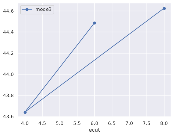
Pandas tables are extremely powerful, and the describe method already gives some useful info about the convergence of the phonon modes. Sometimes, however, we would like to visualize the data to better understand what’s happening:

data_gamma.plot(x="ecut", y="mode3", style="-o");

Let’s plot all the modes in different subplots with:

data_gamma.plot(x="ecut", y=[k for k in data_gamma if k.startswith("mode")], subplots=True, style="-o");

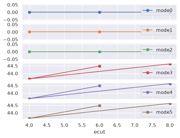
This convergence study thus reveals that our pseudos require ecut >= 6 Ha to get reasonably converged phonon frequencies at \(\Gamma\). In what follows, we assume that the modes at the other \(q\)-points have a similar convergence behaviour, and we use ecut = 6 Ha to keep the computational cost low.

For a quick introduction to pandas, see:

• Pandas cookbook

• Pandas cookbook Chapter 1 Reading data from a csv file

Phonon band structure of AlAs

Now we are finally ready to compute the vibrational spectrum of AlAs. We have already run DFPT calculations at \(\Gamma\) with different values of ecut, and the steps required to get a full band structure are not that different, provided that the following differences are taken into account:

• we need the dynamical matrix \(D(q)\) on a homogeneous mesh, so that anaddb can compute \(D(R)\) via Fourier transform and then the phonon frequencies at arbitrary \(q\)-points via Fourier interpolation;

• AlAs is a polar semiconductor, so we need to include the LO-TO splitting for \(q \rightarrow 0\), which, in turn, requires the DFPT computation of the Born effective charges and of the dielectric constant.

In AbiPy, these concepts are translated into an easy-to-use API in which you pass an initial AbinitInput object, specify the \(q\)-mesh for phonons with ph_ngqpt, and activate the computation of the Born effective charges with the boolean flag with_becs.

Let’s have a look at the code (as usual, there are more comments than lines of code):

from lesson_dfpt import build_flow_alas_phonons
abilab.print_source(build_flow_alas_phonons)

def build_flow_alas_phonons(options):
    """
    Build and return a Flow to compute the dynamical matrix on a (2, 2, 2) qmesh
    as well as DDK and Born effective charges.
    The final DDB with all perturbations will be merged automatically and placed
    in the Flow `outdir` directory.
    """
    scf_input = make_scf_input(ecut=6, ngkpt=(4, 4, 4))
    return flowtk.PhononFlow.from_scf_input("flow_alas_phonons", scf_input,
                                            ph_ngqpt=(2, 2, 2), with_becs=True)

We can finally construct the flow with:

flow_phbands = build_flow_alas_phonons(options=None)

and visualize the connections with:

flow_phbands.get_graphviz()
#flow_phbands.plot_networkx();

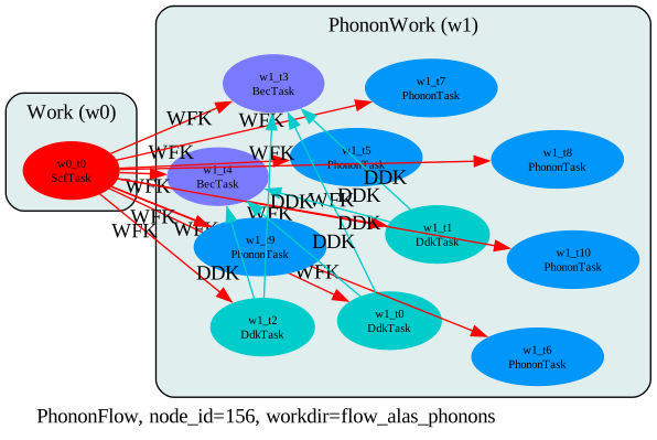
Note that a lot of things are happening under the hood here.

First of all, AbiPy generates PhononTasks only for the \(q\)-points in the irreducible wedge of the Brillouin zone corresponding to ph_ngqpt. Moreover, for a given \(q\)-point, only the irreducible atomic perturbations are explicitly computed, since the other atomic perturbations can be reconstructed by symmetry. Fortunately, you do not have to care about all these technical details, as AbiPy and Abinit automate the whole procedure.

Remember that the \(q\)-point mesh cannot be chosen arbitrarily, since all the \(q\) wavevectors should connect two \(k\)-points of the grid used for the electrons.

It is also worth stressing that the computational cost of the DFPT run depends on the \(q\)-point, since only the symmetries that preserve the \(q\)-point as well as the direction of the perturbation can be employed (calculations at \(\Gamma\) are therefore much faster than at other \(q\)-points).

flow_phbands.get_vars_dataframe("rfphon", "rfatpol", "rfdir", "qpt", "kptopt")

	rfphon	rfatpol	rfdir	qpt	kptopt	class
w0_t0	None	None	None	None	None	ScfTask
w1_t0	None	None	(1, 0, 0)	(0, 0, 0)	2	DdkTask
w1_t1	None	None	(0, 1, 0)	(0, 0, 0)	2	DdkTask
w1_t2	None	None	(0, 0, 1)	(0, 0, 0)	2	DdkTask
w1_t3	1	[1, 1]	[1, 0, 0]	(0, 0, 0)	2	BecTask
w1_t4	1	[2, 2]	[1, 0, 0]	(0, 0, 0)	2	BecTask
w1_t5	1	[1, 1]	[1, 0, 0]	[0.5, 0.0, 0.0]	3	PhononTask
w1_t6	1	[1, 1]	[0, 1, 0]	[0.5, 0.0, 0.0]	3	PhononTask
w1_t7	1	[2, 2]	[1, 0, 0]	[0.5, 0.0, 0.0]	3	PhononTask
w1_t8	1	[2, 2]	[0, 1, 0]	[0.5, 0.0, 0.0]	3	PhononTask
w1_t9	1	[1, 1]	[1, 0, 0]	[0.5, 0.5, 0.0]	3	PhononTask
w1_t10	1	[2, 2]	[1, 0, 0]	[0.5, 0.5, 0.0]	3	PhononTask

Now we can generate the directories and the input files of the Flow. Change lesson_dfpt.py so that build_flow_alas_phonons is called in the main function instead of build_flow_alas_ecut_conv, and run the script to generate the directory with the flow. Finally, use

abirun.py flow_alas_phonons scheduler

to launch the entire calculation.

Post-processing the results

Our flow has completed, and we have the final DDB file with all the \(q\)-points and all the independent atomic perturbations. Let’s open this DDB file with:

ddb = abilab.abiopen("flow_alas_phonons/outdata/out_DDB")
print(ddb)

================================= File Info =================================
Name: out_DDB
Directory: /home/runner/work/abipy_book/abipy_book/abipy_book/dfpt/flow_alas_phonons/outdata
Size: 28.11 kB
Access Time: Wed Sep 30 16:01:41 2026
Modification Time: Wed Sep 30 15:56:52 2026
Change Time: Wed Sep 30 15:56:52 2026

================================= Structure =================================
Full Formula (Al1 As1)
Reduced Formula: AlAs
abc   :   3.970101   3.970101   3.970101
angles:  60.000000  60.000000  60.000000
pbc   :       True       True       True
Sites (2)
  #  SP       a     b     c
---  ----  ----  ----  ----
  0  Al    0     0     0
  1  As    0.25  0.25  0.25

Abinit Spacegroup: spgid: 0, num_spatial_symmetries: 24, has_timerev: True, symmorphic: False

================================== DDB Info ==================================

Number of q-points in DDB: 3
guessed_ngqpt: [2 2 2] (guess for the q-mesh divisions made by AbiPy)
ecut = 6.000000, ecutsm = 0.000000, nkpt = 128, nsym = 24, usepaw = 0
nsppol 1, nspinor 1, nspden 1, ixc = 1, occopt = 1, tsmear = 0.010000

Has total energy: False
Has forces: False
Has stress tensor: False

Has (at least one) atomic perturbation: True
Has (at least one diagonal) electric-field perturbation: True
Has (at least one) Born effective charge: True
Has (all) strain terms: False
Has (all) internal strain terms: False
Has (all) piezoelectric terms: False
Has (all) dynamical quadrupole terms: False

The DdbFile object provides an easy-to-use interface that invokes anaddb to post-process the data stored in the DDB file.

Warning

In order to run ABINIT executables from AbiPy, you need a manager.yml with configuration options. For further details, please consult the TaskManager documentation.

anacompare_phdos, for example, computes the phonon DOS with different \(q\)-meshes. Each mesh is defined by a single integer, nqsmall, that gives the number of divisions used to sample the smallest reciprocal lattice vector. The numbers of divisions along the other directions are chosen so that proportions are preserved:

c = ddb.anacompare_phdos(nqsmalls=[8, 10, 12, 14, 16])

c.plotter.combiplotly();

A 16x16x16 \(q\)-mesh with the tetrahedron method gives a well converged phonon DOS.

The anaget_phbst_and_phdos_files method computes the phonon band structure on an automatically defined \(q\)-path as well as the phonon DOS:

phbst_file, phdos_file = ddb.anaget_phbst_and_phdos_files(ndivsm=10, nqsmall=16, lo_to_splitting=False)

# Extract the phonon bands and the phonon DOS from phbst_file and phdos_file
phbands = phbst_file.phbands
phdos = phdos_file.phdos

Let’s plot the phonon bands:

phbands.plotly(template="plotly_dark");

as well as the high-symmetry \(q\)-path:

phbands.qpoints.plotly();

Do you see the two strange dips of the highest phonon band at the \(\Gamma\) point? They are due to the lack of LO-TO splitting in the anaddb treatment of the first list of vectors. See also the discussion in the second DFPT lesson.

For years, Abinit users had to manually patch the output frequencies to include the LO-TO splitting. These days are finally gone, and we can plot the LO-TO splitting with AbiPy by just setting lo_to_splitting=True:

phbst_file, phdos_file = ddb.anaget_phbst_and_phdos_files(ndivsm=10, nqsmall=16, lo_to_splitting=True)

# Extract the phonon bands and the phonon DOS from phbst_file and phdos_file
phbands = phbst_file.phbands
phdos = phdos_file.phdos

#phbst_file.phbands.qpoints.plot();

The band structure plot now correctly shows the non-analytical behaviour around \(\Gamma\):

phbands.plotly();

Warning

lo_to_splitting=True works only if the DDB contains the Born effective charges and the dielectric constant, which must be computed in the Abinit run.

To plot bands and DOS on the same figure:

phbands.plotly_with_phdos(phdos);

The PhdosFile contains the phonon frequencies and the displacement vectors, as well as the decomposition of the total DOS into the contributions of the different types of atoms in the unit cell. This means that one can plot the type-projected phonon DOS with:

phdos_file.plotly_pjdos_type(title="AlAs type-projected phonon DOS");

and it is even possible to plot fatbands and type-projected DOS on the same figure with:

phbands.plotly_fatbands(phdos_file=phdos_file);

The highest-frequency modes have a strong Al character, while the low-frequency modes originate from As. This behaviour is somewhat expected. Could you explain it in terms of a simple physical model?

Macroscopic dielectric tensor and Born effective charges

Our calculation includes the response of the system to an external electric field. The code below extracts the macroscopic dielectric tensor (emacro) and the Born effective charges (becs) from the DDB file:

emacro, becs = ddb.anaget_epsinf_and_becs()

emacro

	x	y	z
x	10.396165	0.000000	0.000000
y	0.000000	10.396165	0.000000
z	0.000000	0.000000	10.396165

becs

	element	site_index	frac_coords	wyckoff	xx	yy	zz	xy	xz	yx	yz	zx	zy
0	Al	0	[0.0, 0.0, 0.0]	1a	2.168053	2.168053	2.168053	0.0	-2.087488e-19	0.0	-2.087488e-19	0.0	0.0
1	As	1	[0.25, 0.25, 0.25]	1d	-2.168053	-2.168053	-2.168053	0.0	2.087488e-19	0.0	2.087488e-19	0.0	0.0

As explained in the references, the Born effective charges must fulfill the charge neutrality sum rule. This rule is usually broken by the discretization introduced by the FFT mesh, and anaddb enforces it if chneut is set to 1 (default behaviour). Let’s check it out!

print(becs)

Ze effective charges in Cartesian coordinates:
  element  site_index         frac_coords wyckoff        xx        yy        zz   xy            xz   yx            yz   zx   zy
0      Al           0     [0.0, 0.0, 0.0]      1a  2.168053  2.168053  2.168053  0.0 -2.087488e-19  0.0 -2.087488e-19  0.0  0.0
1      As           1  [0.25, 0.25, 0.25]      1d -2.168053 -2.168053 -2.168053  0.0  2.087488e-19  0.0  2.087488e-19  0.0  0.0

Let’s repeat the same calculation without enforcing the sum rule:

emacro, becs_chneut0 = ddb.anaget_epsinf_and_becs(chneut=0)
print(becs_chneut0)

Ze effective charges in Cartesian coordinates:
  element  site_index         frac_coords wyckoff        xx        yy        zz   xy            xz   yx            yz   zx   zy
0      Al           0     [0.0, 0.0, 0.0]      1a  2.127295  2.127295  2.127295  0.0  8.199282e-20  0.0  8.199282e-20  0.0  0.0
1      As           1  [0.25, 0.25, 0.25]      1d -2.208811 -2.208811 -2.208811  0.0  4.994904e-19  0.0  4.994904e-19  0.0  0.0

Thermodynamic properties within the harmonic approximation

The thermodynamic properties of an ensemble of non-interacting phonons can be expressed in terms of integrals of the DOS:

(8)\[\begin{equation} %\label{eq:helmholtz} \Delta F = 3nNk_BT\int_{0}^{\omega_L}\text{ln}\left(2\text{sinh}\frac{\hbar\omega}{2k_BT}\right)g(\omega)d\omega \end{equation}\]

(9)\[\begin{equation} %\label{eq:free_en} \Delta E = 3nN\frac{\hbar}{2}\int_{0}^{\omega_L}\omega\text{coth}\left(\frac{\hbar\omega}{2k_BT}\right)g(\omega)d\omega \end{equation}\]

(10)\[\begin{equation} %\label{eq:c_v} C_v = 3nNk_B\int_{0}^{\omega_L}\left(\frac{\hbar\omega}{2k_BT}\right)^2\text{csch}^2\left(\frac{\hbar\omega}{2k_BT}\right)g(\omega)d\omega \end{equation}\]

(11)\[\begin{equation} %\label{eq:entropy} S = 3nNk_B\int_{0}^{\omega_L}\left(\frac{\hbar\omega}{2k_BT}\text{coth}\left(\frac{\hbar\omega}{2k_BT}\right) - \text{ln}\left(2\text{sinh}\frac{\hbar\omega}{2k_BT}\right)\right)g(\omega)d\omega, \end{equation}\]

where \(k_B\) is the Boltzmann constant.

This is a reasonable approximation, especially in the low-temperature regime, where anharmonic effects can be neglected.

Let’s plot the vibrational contributions to the thermodynamic properties as a function of \(T\):

phdos.plotly_harmonic_thermo();

Exercises

• Our first phonon band structure has been computed with a (4, 4, 4) \(k\)-mesh for the electrons and a (2, 2, 2) \(q\)-mesh for phonons. You may try to increase the density of \(k\)-points/\(q\)-points to see if this change affects the final results.

• Why do you get an error from AbiPy if you try ngkpt = (4, 4, 4) and ngqpt = (3, 3, 3)?