Base3 lesson (silicon)

Base3 lesson (silicon)#

Third (basic) lesson with Abinit and AbiPy

Crystalline silicon.

This lesson shows how to compute the following physical properties of an insulator:

the total energy
the lattice parameter
the Kohn-Sham band structure

You will learn about the use of k-points, as well as the smearing of the plane-wave kinetic energy cut-off.

This tutorial complements the standard ABINIT tutorial on silicon. Here, we demonstrate powerful flow and visualization procedures. Still, some basic understanding of how ABINIT works as a stand-alone code is a prerequisite. Also, to fully benefit from this AbiPy tutorial, you should have followed the more basic AbiPy tutorials, as suggested in the introduction page.

Warning

In order to run ABINIT executables from AbiPy, you need a manager.yml with configuration options. For further details, please consult the TaskManager documentation.

import numpy as np

import warnings
warnings.filterwarnings("ignore")  # Ignore warnings

from abipy import abilab
abilab.enable_notebook() # This line tells AbiPy we are running inside a notebook

# This line configures matplotlib to show figures embedded in the notebook.
# Replace `inline` with `notebook` in classic notebook
%matplotlib inline

# Option available in jupyterlab. See https://github.com/matplotlib/jupyter-matplotlib
#%matplotlib widget

Note

AbiPy provides two different APIs to produce figures, with either matplotlib or plotly. In this tutorial, we use the plotly API as much as possible, although it should be noted that not all the plotting methods have been ported to plotly yet.

AbiPy uses a relatively simple rule to differentiate between the two plotting libraries: if an object provides an obj.plot method producing a matplotlib plot, the corresponding native plotly version (if available) is named obj.plotly. Note that plotly requires a web browser, hence the matplotlib version is still valuable if you need to visualize results on machines on which only an X server is available.

In AbiPy versions greater than 0.9, you can try to convert the matplotlib figures produced by plot methods into Plotly figures using the optional argument plotly=True, although the result is not always guaranteed.

Computing the total energy of silicon at fixed number of k-points#

Our goal is to study the convergence of the total energy of silicon with respect to the number of \(k\)-points. So we start by defining a function that generates a Flow of SCF calculations by looping over a predefined list of ngkpt values. The crystalline structure is initialized from a CIF file, while other parameters such as the cutoff energy ecut are fixed:

from lesson_base3 import build_ngkpt_flow
abilab.print_source(build_ngkpt_flow)

def build_ngkpt_flow(options):
    """
    Crystalline silicon: computation of the total energy
    Convergence with respect to the number of k points. Similar to tbase3_3.in

    Args:
        options: Command line options.

    Return:
        Abinit Flow object.
    """
    # Definition of the different grids
    ngkpt_list = [(2, 2, 2), (4, 4, 4), (6, 6, 6), (8, 8, 8)]

    # These shifts will be the same for all grids
    shiftk = [float(s) for s in "0.5 0.5 0.5 0.5 0.0 0.0 0.0 0.5 0.0 0.0 0.0 0.5".split()]

    # Build MultiDataset object (container of `ndtset` inputs).
    # Structure is initialized from CIF file.
    multi = abilab.MultiDataset(structure=abidata.cif_file("si.cif"),
                                pseudos=abidata.pseudos("14si.pspnc"), ndtset=len(ngkpt_list))

    # These variables are the same in each input.
    multi.set_vars(ecut=8, toldfe=1e-6, diemac=12.0, iomode=3)

    # Each input has its own value of `ngkpt`. shiftk is constant.
    for i, ngkpt in enumerate(ngkpt_list):
        multi[i].set_kmesh(ngkpt=ngkpt, shiftk=shiftk)

    workdir = options.workdir if (options and options.workdir) else "flow_base3_ngkpt"

    # Split the inputs by calling multi.datasets() and pass the list of inputs to Flow.from_inputs.
    return flowtk.Flow.from_inputs(workdir, inputs=multi.split_datasets())

Let’s call the function to build the flow:

flow = build_ngkpt_flow(options=None)

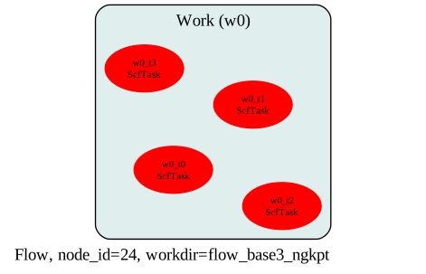
In total, we have four ScfTasks that will be executed in the flow_base3_ngkpt directory:

flow.get_graphviz()

../_images/149692c84dadbcc38358735cdd9807c112c3026ee62dd2bac8037e1ecea79f98.svg

This is the input of the first task w0_t0:

flow[0][0].input

##############################################
#### SECTION: basic
##############################################
ecut 8
toldfe 1e-06
ngkpt 2 2 2
kptopt 1
nshiftk 4
shiftk
0.5 0.5 0.5
0.5 0.0 0.0
0.0 0.5 0.0
0.0 0.0 0.5
##############################################
#### SECTION: dev
##############################################
iomode 3
##############################################
#### SECTION: files
##############################################
indata_prefix indata/in
tmpdata_prefix tmpdata/tmp
outdata_prefix outdata/out
pseudos /home/runner/work/abipy_book/abipy_book/abipy/abipy/data/pseudos/14si.pspnc
##############################################
#### SECTION: gstate
##############################################
diemac 12.0
##############################################
#### STRUCTURE
##############################################
natom 2
ntypat 1
typat 1 1
znucl 14
xred
0.0000000000 0.0000000000 0.0000000000
0.2500000000 0.2500000000 0.2500000000
acell 1.0 1.0 1.0
rprim
6.3285005287 0.0000000000 3.6537614838
2.1095001762 5.9665675181 3.6537614838
0.0000000000 0.0000000000 7.3075229676

and these are the ngkpt divisions of the \(k\)-mesh for the four different calculations:

for task in flow.iflat_tasks():
    print(task.pos_str, "uses ngkpt:", task.input["ngkpt"])

w0_t0 uses ngkpt: (2, 2, 2)
w0_t1 uses ngkpt: (4, 4, 4)
w0_t2 uses ngkpt: (6, 6, 6)
w0_t3 uses ngkpt: (8, 8, 8)

We can achieve the same goal more concisely with:

flow.get_vars_dataframe("ngkpt", "ecut")

	ngkpt	ecut	class
w0_t0	(2, 2, 2)	8	ScfTask
w0_t1	(4, 4, 4)	8	ScfTask
w0_t2	(6, 6, 6)	8	ScfTask
w0_t3	(8, 8, 8)	8	ScfTask

At this point, we could run the flow in the notebook by just calling:

flow.make_scheduler().start()

or, alternatively, execute the lesson_base3.py script to build the directory with the flow and then use:

abirun.py flow_base3_ngkpt scheduler

inside the terminal.

Analysis of the results#

We could use the API provided by the flow to extract the total energies from the GSR files, with something like:

nkpt_list, ene_list = [], []
for task in flow.iflat_tasks():
    with task.open_gsr() as gsr:
        nkpt_list.append(gsr.nkpt)
        ene_list.append(gsr.energy)

# Assuming values are already sorted wrt nkpt
import matplotlib.pyplot as plt
plt.plot(nkpt_list, ene_list, marker="o");

but it is much easier to create a GsrRobot that does the work for us:

robot_enekpt = abilab.GsrRobot.from_dir("flow_base3_ngkpt")
robot_enekpt

w0/t0/outdata/out_GSR.nc
w0/t3/outdata/out_GSR.nc
w0/t2/outdata/out_GSR.nc
w0/t1/outdata/out_GSR.nc

Next, we generate a pandas DataFrame with the most important results, and show how to use the pandas API to analyze the data:

ene_table = robot_enekpt.get_dataframe()
ene_table.keys()

Index(['formula', 'natom', 'alpha', 'beta', 'gamma', 'a', 'b', 'c', 'volume',
       'abispg_num', 'spglib_symb', 'spglib_num', 'spglib_lattice_type',
       'energy', 'energy_per_atom', 'pressure', 'max_force', 'ecut',
       'pawecutdg', 'tsmear', 'nkpt', 'nsppol', 'nspinor', 'nspden'],
      dtype='str')

The dataframe contains several columns, but we are mainly interested in the number of \(k\)-points nkpt and in the energy (given in eV). Let’s massage the data a bit to facilitate the post-processing:

# We are gonna plot f(nkpt) so let's sort the rows first.
ene_table.sort_values(by="nkpt", inplace=True)

# Add a column with energies in Ha and another column with the difference wrt to the last point.
ene_table["energy_Ha"] = ene_table["energy"] * abilab.units.eV_to_Ha
ene_table["ediff_Ha"] = ene_table["energy_Ha"] - ene_table["energy_Ha"][-1]

---------------------------------------------------------------------------
KeyError                                  Traceback (most recent call last)
File /usr/share/miniconda/envs/abipy/lib/python3.14/site-packages/pandas/core/indexes/base.py:3641, in Index.get_loc(self, key)
   3640 try:
-> 3641     return self._engine.get_loc(casted_key)
   3642 except KeyError as err:

File pandas/_libs/index.pyx:168, in pandas._libs.index.IndexEngine.get_loc()
--> 168 'Could not get source, probably due dynamically evaluated source code.'

File pandas/_libs/index.pyx:176, in pandas._libs.index.IndexEngine.get_loc()
--> 176 'Could not get source, probably due dynamically evaluated source code.'

File pandas/_libs/index.pyx:583, in pandas._libs.index.StringObjectEngine._check_type()
--> 583 'Could not get source, probably due dynamically evaluated source code.'

KeyError: -1

The above exception was the direct cause of the following exception:

KeyError                                  Traceback (most recent call last)
Cell In[10], line 6
      2 ene_table.sort_values(by="nkpt", inplace=True)
      3 
      4 # Add a column with energies in Ha and another column with the difference wrt to the last point.
      5 ene_table["energy_Ha"] = ene_table["energy"] * abilab.units.eV_to_Ha
----> 6 ene_table["ediff_Ha"] = ene_table["energy_Ha"] - ene_table["energy_Ha"][-1]

File /usr/share/miniconda/envs/abipy/lib/python3.14/site-packages/pandas/core/series.py:959, in Series.__getitem__(self, key)
    954     key = unpack_1tuple(key)
    956 elif key_is_scalar:
    957     # Note: GH#50617 in 3.0 we changed int key to always be treated as
    958     #  a label, matching DataFrame behavior.
--> 959     return self._get_value(key)
    961 # Convert generator to list before going through hashable part
    962 # (We will iterate through the generator there to check for slices)
    963 if is_iterator(key):

File /usr/share/miniconda/envs/abipy/lib/python3.14/site-packages/pandas/core/series.py:1046, in Series._get_value(self, label, takeable)
   1043     return self._values[label]
   1045 # Similar to Index.get_value, but we do not fall back to positional
-> 1046 loc = self.index.get_loc(label)
   1048 if is_integer(loc):
   1049     return self._values[loc]

File /usr/share/miniconda/envs/abipy/lib/python3.14/site-packages/pandas/core/indexes/base.py:3648, in Index.get_loc(self, key)
   3643     if isinstance(casted_key, slice) or (
   3644         isinstance(casted_key, abc.Iterable)
   3645         and any(isinstance(x, slice) for x in casted_key)
   3646     ):
   3647         raise InvalidIndexError(key) from err
-> 3648     raise KeyError(key) from err
   3649 except TypeError:
   3650     # If we have a listlike key, _check_indexing_error will raise
   3651     #  InvalidIndexError. Otherwise we fall through and re-raise
   3652     #  the TypeError.
   3653     self._check_indexing_error(key)

KeyError: -1

before printing a subset of the columns with the syntax:

ene_table[["nkpt", "energy", "energy_Ha", "ediff_Ha"]]

If you do not like tables and prefer figures, use:

ene_table.plot(x="nkpt", y=["energy_Ha", "ediff_Ha", "pressure"], style="-o", subplots=True);

The difference between dataset 3 and dataset 4 is rather small. Even dataset 2 gives an accuracy of about 0.0001 Ha. So, our converged value for the total energy (at fixed acell and ecut) is -8.8726 Ha.

Now that we have learned a bit about pandas DataFrames, we can finally reveal that the AbiPy robots already provide methods to perform this kind of convergence study, so that we do not need to manipulate pandas dataframes explicitly. For example, we can perform the same analysis with a single line:

robot_enekpt.plot_gsr_convergence(sortby="nkpt");

We can also pass a function that the robot calls to compute the values along the x-axis and sort the results. The docstring of the function is used as the label of the x-axis:

def inv_nkpt(abifile):
    r"""$\dfrac{1}{nkpt}$"""
    return 1 / abifile.nkpt

robot_enekpt.plot_gsr_convergence(sortby=inv_nkpt);

#robot_enekpt.plot_lattice_convergence(sortby="nkpt");

Determination of the lattice parameters#

At this point, the original Abinit tutorial proceeds with a convergence study of the optimized lattice parameters as a function of the \(k\)-point sampling. In AbiPy, we only need to build relaxation tasks with slightly different inputs in which only ngkpt is changed.

from lesson_base3 import build_relax_flow
abilab.print_source(build_relax_flow)

relax_flow = build_relax_flow(options=None)
relax_flow.get_graphviz()

Important

If you want to run the flow from the shell, open lesson_base3.py and change the main function so that it calls build_relax_flow instead of build_ngkpt_flow.

This is our first structural relaxation with AbiPy, and it gives us the opportunity to introduce the HIST.nc file. This file stores the history of the relaxation (energies, forces, stresses, lattice parameters and atomic positions at the different relaxation steps).

As usual, we use abiopen to open an Abinit file object:

hist = abilab.abiopen("flow_base3_relax/w0/t1/outdata/out_HIST.nc")
print(hist)

To plot the evolution of the most important physical quantities, use:

hist.plotly(template="plotly_dark");

hist_robot = abilab.HistRobot.from_dir("flow_base3_relax")

hist_table = hist_robot.get_dataframe()

There are several entries in the DataFrame:

hist_table.keys()

Let’s select some of them with:

hist_table[["alpha", "a", "final_energy", "final_pressure", "num_steps"]]

and plot the evolution of important physical properties extracted from the two files:

hist_robot.gridplot(what_list=["energy", "abc", "pressure", "forces"]);

We can also compare the two structural relaxations with:

hist_robot.combiplot();

Unfortunately, the HIST.nc file does not have enough metadata. In particular, we would like to have information about the \(k\)-point sampling so that we can analyze the convergence of the optimized lattice parameters with respect to nkpt. Fortunately, the GSR.nc file has all the information we need, and it is just a matter of replacing the HistRobot with a GsrRobot:

with abilab.GsrRobot.from_dir("flow_base3_relax") as relkpt_robot:
    relax_table = relkpt_robot.get_dataframe().sort_values(by="nkpt")
    dfs = relkpt_robot.get_structure_dataframes()

relax_table[["energy", "a", "pressure", "max_force", "pressure"]]

Plotting the energy, the lattice parameter a and the pressure (in GPa) vs nkpt is really a piece of cake!

relax_table.plot(x="nkpt", y=["energy", "a", "pressure"], subplots=True);

Alternatively, one can use the GsrRobot API:

relkpt_robot.plot_gsr_convergence(sortby="nkpt");

relkpt_robot.plot_lattice_convergence(what_list=["a"], sortby="nkpt");

In what follows, we fix the acell parameters to the theoretical value of 3*10.216, as well as the grid of \(k\)-points (the 4x4x4 FCC grid, equivalent to an 8x8x8 Monkhorst-Pack grid). We will ask for 8 bands (4 valence and 4 conduction).

Computing the band structure#

A band structure can be computed by solving the Kohn-Sham equation for several \(k\)-points along the high-symmetry lines of the Brillouin zone. The potential that enters the Kohn-Sham equation must be derived from a previous self-consistent calculation, and does not vary during the scan of the different \(k\)-point lines.

This is our first Flow with dependencies, in the sense that the band structure calculation must be connected to a previous SCF run. Fortunately, AbiPy provides a factory function to generate this kind of workflow, so we only need to focus on the definition of the two inputs:

from lesson_base3 import build_ebands_flow
abilab.print_source(build_ebands_flow)

The Flow consists of a single Work with two Tasks (an ScfTask on a \(k\)-mesh and an NscfTask on the \(k\)-path).

ebands_flow = build_ebands_flow(options=None)
ebands_flow.get_graphviz()

Note

If you want to run the flow from the shell, open lesson_base3.py and change the main function so that it calls build_ebands_flow.

Let’s extract the band structure from the GSR.nc file produced by the NscfTask:

with abilab.abiopen("flow_base3_ebands/w0/t1/outdata/out_GSR.nc") as gsr:
    ebands_kpath = gsr.ebands

and plot it with:

ebands_kpath.plotly(with_gaps=True);

Visual inspection reveals that the width of the valence band is ~11.8 eV and that the lowest unoccupied state at X is ~0.5 eV higher than the top of the valence band at \(\Gamma\). Bulk silicon is described as an indirect band gap material (this is correct), with a band gap of about 0.5 eV (this is quantitatively quite wrong: the experimental value is 1.17 eV at 25 degrees Celsius, the famous DFT band-gap problem). The minimum of the conduction band is slightly displaced with respect to X.

Unfortunately, AbiPy does not seem to agree with us:

print(ebands_kpath)

The reason is that the Fermi energy in ebands_kpath is not completely consistent with the band structure. The Fermi energy, indeed, has been taken from the previous GS-SCF calculation performed on a shifted \(k\)-mesh that does not include the \(\Gamma\) point, and is therefore underestimated.

To fix this problem, we have to manually set the Fermi energy to the maximum of the valence bands:

ebands_kpath.set_fermie_to_vbm()
print(ebands_kpath)

Now the AbiPy results are consistent with our initial analysis:

ebands_kpath.plot(with_gaps=True);

# We can also plot the k-path in the Brillouin zone with:
#ebands_kpath.kpoints.plotly();

The GSR file produced by the first task contains energies on a homogeneous \(k\)-mesh, so we can compute the DOS by invoking the get_edos method:

with abilab.abiopen("flow_base3_ebands/w0/t0/outdata/out_GSR.nc") as gsr:
    ebands_kmesh = gsr.ebands

edos = ebands_kmesh.get_edos()

and plot the DOS with:

edos.plotly();

where the zero of the energy axis is set to the Fermi level \(\epsilon_F\) obtained by solving:

\[\int_{-\infty}^{\epsilon_F} g(\epsilon)\,d\epsilon = N\]

for \(\epsilon_F\), with \(N\) the number of electrons per unit cell. Note that the DOS is highly sensitive to the sampling of the IBZ and to the value of the broadening, especially in metallic systems.

edos.plotly_dos_idos();

Want to make a nice picture of the band dispersion with a second panel for the DOS?

ebands_kpath.plotly_with_edos(edos);

It is important to stress that each panel in the above figure is aligned with respect to its own Fermi energy, and these values are not necessarily equal:

print(ebands_kpath.fermie, edos.fermie)

We can always plot the bands and the DOS without setting their Fermi energy to zero by using:

ebands_kpath.plotly_with_edos(edos, e0=0);

This figure shows that the bands and the DOS are not perfectly aligned. More specifically, we would expect the DOS to go to zero at the top of the valence band and at the bottom of the conduction band. This problem is essentially due to the relatively large Gaussian broadening. One should therefore compute the DOS with a much denser IBZ mesh and a much smaller broadening to solve this alignment issue.