The SIGRES file (GW)#
This notebook explains how to use AbiPy and matplotlib to visualize the results produced by the GW code.
The self-energy code (optdriver 4) saves the final results in the SIGRES.nc file
while the screening code (optdriver 3) stores the inverse dielectric matrix in the SCR.nc file.
Let’s start by importing the basic modules we will need for this tutorial.
import warnings
warnings.filterwarnings("ignore")  # Ignore warnings

from abipy import abilab
abilab.enable_notebook() # This line tells AbiPy we are running inside a notebook
import abipy.data as abidata

# This line configures matplotlib to show figures embedded in the notebook.
# Replace `inline` with `notebook` in classic notebook
%matplotlib inline

# Option available in jupyterlab. See https://github.com/matplotlib/jupyter-matplotlib
#%matplotlib widget
How to visualize QP corrections#
As usual, we start by opening the netcdf file with abiopen:
sigres = abilab.abiopen(abidata.ref_file("tgw1_9o_DS4_SIGRES.nc"))
print(sigres)
================================= File Info =================================
Name: tgw1_9o_DS4_SIGRES.nc
Directory: /home/runner/work/abipy_book/abipy_book/abipy/abipy/data/refs
Size: 1005.34 kB
Access Time: Thu Jan 15 12:20:36 2026
Modification Time: Thu Jan 15 12:15:09 2026
Change Time: Thu Jan 15 12:15:09 2026

================================= Structure =================================
Full Formula (Si2)
Reduced Formula: Si
abc   :   3.823046   3.823046   3.823046
angles:  60.000000  60.000000  60.000000
pbc   :       True       True       True
Sites (2)
  #  SP       a     b     c
---  ----  ----  ----  ----
  0  Si    0     0     0
  1  Si    0.25  0.25  0.25

Abinit Spacegroup: spgid: 0, num_spatial_symmetries: 48, has_timerev: True, symmorphic: True

============================== Kohn-Sham bands ==============================
Number of electrons: 8.0, Fermi level: 5.951 (eV)
nsppol: 1, nkpt: 6, mband: 100, nspinor: 1, nspden: 1
smearing scheme:  (occopt 1), tsmear_eV: 1.088, tsmear Kelvin: 12631.0
Direct gap:
    Energy: 2.513 (eV)
    Initial state: spin: 0, kpt: [+0.000, +0.000, +0.000], weight: 0.031, band: 3, eig: 5.951, occ: 2.000
    Final state:   spin: 0, kpt: [+0.000, +0.000, +0.000], weight: 0.031, band: 4, eig: 8.464, occ: 0.000
Fundamental gap:
    Energy: 0.570 (eV)
    Initial state: spin: 0, kpt: [+0.000, +0.000, +0.000], weight: 0.031, band: 3, eig: 5.951, occ: 2.000
    Final state:   spin: 0, kpt: [+0.500, +0.500, +0.000], weight: 0.094, band: 4, eig: 6.521, occ: 0.000
Bandwidth: 12.096 (eV)
Valence maximum located at kpt index 5:
    spin: 0, kpt: [+0.000, +0.000, +0.000], weight: 0.031, band: 3, eig: 5.951, occ: 2.000
Conduction minimum located at kpt index 2:
    spin: 0, kpt: [+0.500, +0.500, +0.000], weight: 0.094, band: 4, eig: 6.521, occ: 0.000

TIP: Use `--verbose` to print k-point coordinates with more digits

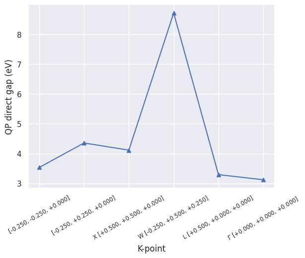
=============================== QP direct gaps ===============================
QP_dirgap: 3.537 (eV) for k-point: [-0.250, -0.250, +0.000], spin: 0
QP_dirgap: 4.357 (eV) for k-point: [-0.250, +0.250, +0.000], spin: 0
QP_dirgap: 4.117 (eV) for k-point: X [+0.500, +0.500, +0.000], spin: 0
QP_dirgap: 8.711 (eV) for k-point: W [-0.250, +0.500, +0.250], spin: 0
QP_dirgap: 3.297 (eV) for k-point: L [+0.500, +0.000, +0.000], spin: 0
QP_dirgap: 3.126 (eV) for k-point: $\Gamma$ [+0.000, +0.000, +0.000], spin: 0


============== QP results for each k-point and spin (all in eV) ==============
K-point: [-0.250, -0.250, +0.000], spin: 0
   band      e0     qpe  qpe_diago   vxcme  sigxme  sigcmee0        vUme  \
0     0  -5.046  -4.760     -4.561 -10.493 -16.549     6.542  1.344e-321
1     1   2.411   2.281      2.238 -11.089 -13.671     2.410  1.344e-321
2     2   4.008   3.867      3.825 -10.689 -12.566     1.694  1.344e-319
3     3   4.008   3.867      3.825 -10.689 -12.566     1.695  1.334e-322
4     4   6.963   7.405      7.523  -9.434  -5.330    -3.544  8.053e-322
5     5   8.979   9.462      9.594  -9.212  -4.504    -4.093  1.636e-152
6     6  11.702  12.132     12.276 -10.569  -5.276    -4.719  1.344e-321
7     7  11.702  12.133     12.278 -10.569  -5.276    -4.717  1.344e-321

     ze0
0  0.589
1  0.751
2  0.768
3  0.769
4  0.789
5  0.786
6  0.748
7  0.748

K-point: [-0.250, +0.250, +0.000], spin: 0
   band      e0     qpe  qpe_diago   vxcme  sigxme  sigcmee0        vUme  \
0     0  -4.064  -3.960     -3.904 -10.617 -16.264     5.808  1.340e-319
1     1   0.418   0.303      0.258 -10.811 -14.348     3.376   0.000e+00
2     2   2.088   1.979      1.944 -10.067 -12.427     2.216   0.000e+00
3     3   4.590   4.437      4.391 -10.912 -12.687     1.576   0.000e+00
4     4   8.311   8.793      8.925  -9.604  -5.066    -3.924  5.774e-313
5     5  10.711  11.188     11.335 -10.115  -4.841    -4.649  1.334e-322
6     6  11.052  11.455     11.573 -10.233  -5.401    -4.310  2.668e-322
7     7  11.990  12.395     12.526  -9.894  -4.357    -5.001   0.000e+00

     ze0
0  0.652
1  0.723
2  0.758
3  0.770
4  0.786
5  0.764
6  0.773
7  0.756

K-point: X [+0.500, +0.500, +0.000], spin: 0
   band      e0     qpe  qpe_diago   vxcme  sigxme  sigcmee0        vUme  \
0     0  -1.936  -1.940     -1.947 -10.762 -15.448     4.680  1.732e-312
1     1  -1.936  -1.944     -1.942 -10.762 -15.448     4.675  6.719e-322
2     2   3.030   2.851      2.795 -10.568 -12.966     2.163   0.000e+00
3     3   3.030   2.851      2.795 -10.568 -12.966     2.163  5.774e-313
4     4   6.521   6.968      7.084  -9.078  -5.038    -3.478  5.774e-313
5     5   6.521   6.969      7.084  -9.078  -5.038    -3.477  1.334e-322
6     6  15.976  16.184     16.280 -10.528  -3.786    -6.438   0.000e+00
7     7  15.976  16.185     16.282 -10.528  -3.786    -6.437  5.385e-322

     ze0
0  0.700
1  0.701
2  0.762
3  0.761
4  0.795
5  0.795
6  0.685
7  0.684

K-point: W [-0.250, +0.500, +0.250], spin: 0
   band      e0     qpe  qpe_diago   vxcme  sigxme  sigcmee0        vUme  \
0     0  -1.760  -1.773     -1.808 -10.873 -15.503     4.611  6.722e-320
1     1  -1.760  -1.793     -1.778 -10.873 -15.503     4.582  1.334e-322
2     2   1.982   1.867      1.830  -9.991 -12.434     2.290   0.000e+00
3     3   1.982   1.867      1.830  -9.991 -12.434     2.290   0.000e+00
4     4  10.159  10.578     10.696  -9.647  -4.967    -4.142  6.722e-320
5     5  10.159  10.577     10.697  -9.647  -4.967    -4.143   0.000e+00
6     6  10.902  11.366     11.509 -10.031  -4.701    -4.722   0.000e+00
7     7  10.902  11.366     11.509 -10.031  -4.701    -4.722   0.000e+00

     ze0
0  0.691
1  0.691
2  0.757
3  0.757
4  0.779
5  0.779
6  0.764
7  0.764

K-point: L [+0.500, +0.000, +0.000], spin: 0
   band      e0     qpe  qpe_diago   vxcme  sigxme  sigcmee0        vUme  \
0     0  -3.760  -3.647     -3.578 -10.759 -16.296     5.719   0.000e+00
1     1  -1.137  -1.182     -1.198 -10.178 -14.330     4.091  5.543e-311
2     2   4.726   4.559      4.509 -11.006 -12.812     1.588   0.000e+00
3     3   4.726   4.559      4.509 -11.006 -12.812     1.588   0.000e+00
4     4   7.408   7.856      7.978 -10.054  -5.736    -3.748   0.000e+00
5     5   9.251   9.772      9.915  -9.698  -4.959    -4.074   0.000e+00
6     6   9.251   9.771      9.916  -9.698  -4.959    -4.075   0.000e+00
7     7  13.458  13.754     13.847  -8.011  -2.413    -5.210   0.000e+00

     ze0
0  0.623
1  0.737
2  0.772
3  0.772
4  0.785
5  0.783
6  0.783
7  0.760

K-point: $\Gamma$ [+0.000, +0.000, +0.000], spin: 0
   band     e0    qpe  qpe_diago   vxcme  sigxme  sigcmee0  vUme    ze0
0     0 -6.145 -5.719     -5.412 -10.388 -16.893     7.239   0.0  0.581
1     1  5.951  5.806      5.764 -11.253 -12.628     1.188   0.0  0.777
2     2  5.951  5.806      5.764 -11.253 -12.628     1.188   0.0  0.777
3     3  5.951  5.806      5.764 -11.253 -12.628     1.187   0.0  0.777
4     4  8.464  8.931      9.065 -10.042  -5.563    -3.878   0.0  0.777
5     5  8.464  8.932      9.066 -10.042  -5.563    -3.877   0.0  0.777
6     6  8.464  8.933      9.067 -10.042  -5.563    -3.876   0.0  0.778
7     7  9.205  9.664      9.798 -10.748  -5.734    -4.421   0.0  0.773
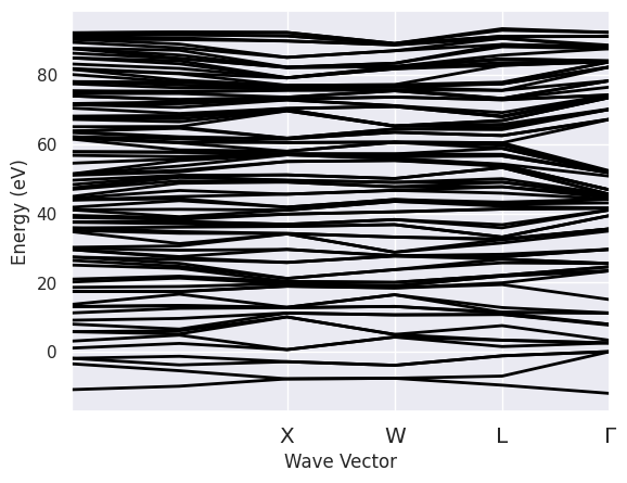
Let’s have a look at the KS energies used to compute the Green’s function \(G_0\), the RPA screening \(W_0\) and the \(G_0W_0\) self-energy:
sigres.ebands.plot();
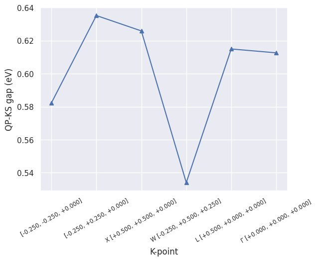
The SIGRES file contains the KS as well as the QP direct gaps for all the k-points included in the calculation (kptgw). To plot the difference QP - KS, use:
sigres.plot_qpgaps();
For the absolute QP gaps:
sigres.plot_qpgaps(plot_qpmks=False);
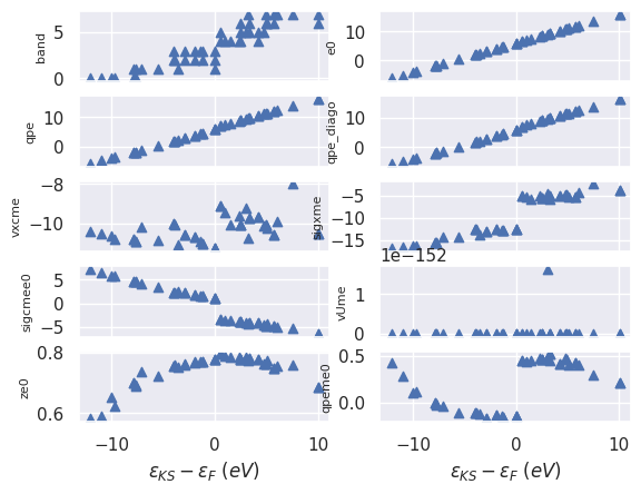
To plot the QP results as a function of the initial KS energy:
sigres.plot_qps_vs_e0(); #tight_layout=True);
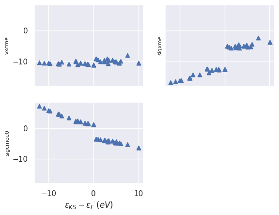
and use with_fields to filter the quantity of interest:
sigres.plot_qps_vs_e0(with_fields=["vxcme", "sigxme", "sigcmee0"], sharey=True);
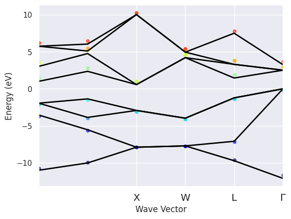
To plot the QP energies on top of the KS energies used in the SIGMA run:
sigres.plot_qpbands_ibz();
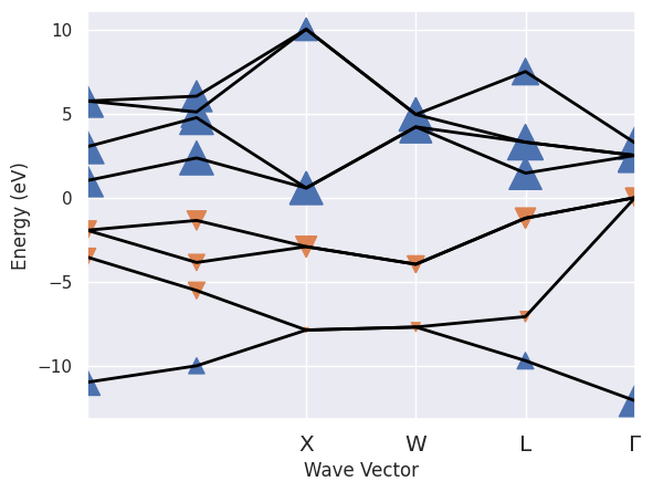
To plot the KS band structure with markers whose size is proportional to the QP correction and whose direction gives the sign of the correction:
sigres.plot_ksbands_with_qpmarkers(fact=1000);
We can also plot the \(<\Psi^{KS}_{mk}\,|\,\Psi^{QP}_{nk}>\) coefficients for given spin and k-point:
sigres.plot_eigvec_qp(spin=0, kpoint=0);
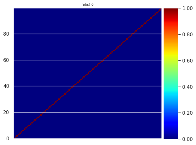
In this case, we have a diagonal matrix because the wavefunctions are not updated (\(G_0W_0\)). The scenario is completely different if you start to perform self-consistent calculations with update of the QP amplitudes.
Plotting the spectral function#
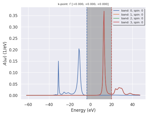
This example shows how to plot the \(G_0W_0\) spectral functions \(A(\omega)\) at the \(\Gamma\) point. See also lesson tgw2_4
with abilab.abiopen(abidata.ref_file("al_g0w0_sigmaw_SIGRES.nc")) as al_sigres:
    # Plot A(w) for the first spin, the gamma point, and bands in [0,1,2,3]
    al_sigres.plot_spectral_functions();
Analyzing multiple SIGRES files with robots#
To analyze the convergence of the QP results, we can use the SigresRobot. Let’s build our robot from a list of SIGRES files.
# List of SIGRES files computed with different values of nband.
filenames = [
    "si_g0w0ppm_nband10_SIGRES.nc",
    "si_g0w0ppm_nband20_SIGRES.nc",
    "si_g0w0ppm_nband30_SIGRES.nc",
]

filepaths = [abidata.ref_file(fname) for fname in filenames]

robot = abilab.SigresRobot.from_files(filepaths)
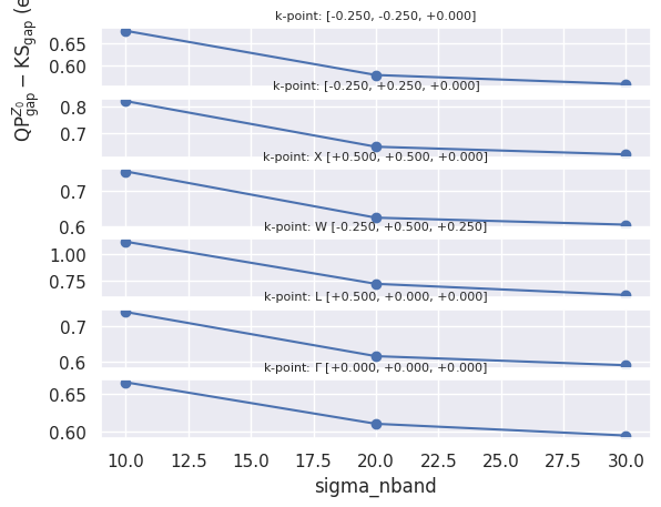
Then we plot the convergence of the QP direct gap as a function of the number of bands in the self-energy for all the k-points available in the netcdf files:
robot.plot_qpgaps_convergence(sortby="sigma_nband", sharey=False);
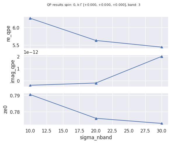
If we are interested in the convergence of the real/imaginary part of the self-energy and of the renormalization factor …
robot.plot_qpdata_conv_skb(spin=0, kpoint=(0, 0, 0), band=3, sortby="sigma_nband");
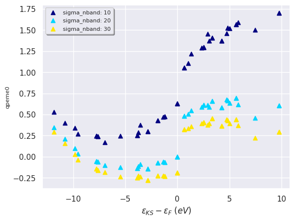
We can also plot the QP data as a function of the KS energies on the same figure with:
robot.plot_qpfield_vs_e0("qpeme0", sortby="sigma_nband");
#robot.get_qpgaps_dataframe(spin=0, kpoint=(0, 0, 0))

