Tasks, Workflows and Flow

In this notebook, we discuss some of the basic concepts used in AbiPy to automate ab-initio calculations. In particular, we focus on the following three objects:

• Task

• Work

• Flow

The Task represents the most elementary step of the automatic workflow. Roughly speaking, it corresponds to the execution of a single Abinit calculation without multiple datasets.

From the point of view of AbiPy, a calculation consists of a set of Tasks connected by dependencies. Each task has a list of files that are needed to start the calculation, and a list of files that are produced at the end of the run.

Some of the input files needed by a Task must be provided by the user in the form of Abinit input variables (e.g. crystalline structure, pseudopotentials), while other inputs may be produced by other tasks. When a Task B requires the output file DEN of another task A, we say that B depends on A through a DEN file, and we express this dependency with the dictionary:

B_deps = {A: "DEN"}

To clarify this point, let’s take a standard KS band structure calculation as an example. In this case, we have an initial ScfTask that solves the KS equations self-consistently to produce a DEN file. The density is then used by a second NscfTask to compute a band structure on an arbitrary list of \(k\)-points. The NscfTask therefore depends on the ScfTask, in the sense that it cannot be executed until the ScfTask has completed and produced the DEN file.

Now that we have clarified the concept of Task, we can finally turn to Works and Flows. A Work can be seen as a list of Tasks, while a Flow is essentially a list of Work objects. Works are usually used to group tasks that are connected to each other, while Flows are the final objects that are executed. The Flow provides an easy-to-use high-level API to perform common operations such as launching the actual jobs, checking the status of the Tasks, correcting problems, etc.

AbiPy provides several tools, the so-called factory functions, to generate Flows for typical calculations. This means that you do not need to understand all the technical details of the Python implementation. In many cases, indeed, we already provide a Work or a Flow that automates the whole calculation, and you only need to provide the correct list of input files. Obviously, this list must be consistent with the kind of Flow/Work you are using. For instance, you should not pass a list of inputs for a band structure calculation to a Work that is expected to compute phonons with DFPT!

All the Works and Tasks of a flow are created and executed inside the working directory (workdir), which is usually specified by the user when creating the Flow object. AbiPy creates the workdirs of the different Works/Tasks when the Flow is executed for the first time.

Each Task contains a set of input variables that will be used to generate the Abinit input file. This input must be provided by the user when creating the Task. Fortunately, AbiPy provides the AbinitInput object to facilitate the creation of such input. Once you have an AbinitInput, you can create the corresponding Task with the (pseudo) code:

new_task = Task(abinit_input_object)

The Task provides several methods for monitoring the status of the calculation and post-processing the results. Note that the concept of dependency is not limited to files. All the Tasks in the flow are connected and can interact with each other. This allows programmers to implement Python functions that will be invoked by the framework at run time. For example, one can implement a Task that fetches the relaxed structure from a previous Task and uses this configuration to start a DFPT calculation.

In the next section, we discuss how to construct a Flow for band structure calculations with a high-level interface that only requires the input files. This example allows us to discuss the most important methods of the Flow.

Building a Flow for band structure calculations

Let’s start by creating a function that produces two input files. The first input is a standard self-consistent ground-state run. The second input uses the density produced in the first run to perform a non-self-consistent band structure calculation.

# This line configures matplotlib to show figures embedded in the notebook.
# Replace `inline` with `notebook` in classic notebook
%matplotlib inline

# Option available in jupyterlab. See https://github.com/matplotlib/jupyter-matplotlib
#%matplotlib widget

import warnings
warnings.filterwarnings("ignore") # to get rid of deprecation warnings

from abipy import abilab
import os
import abipy.flowtk as flowtk
import abipy.data as abidata

def make_scf_nscf_inputs():
    """Build ands return the input files for the GS-SCF and the GS-NSCF tasks."""
    multi = abilab.MultiDataset(structure=abidata.cif_file("si.cif"),
                                pseudos=abidata.pseudos("14si.pspnc"), ndtset=2)

    # Set global variables (dataset1 and dataset2)
    multi.set_vars(ecut=6, nband=8)

    # Dataset 1 (GS-SCF run)
    multi[0].set_kmesh(ngkpt=[8,8,8], shiftk=[0,0,0])
    multi[0].set_vars(tolvrs=1e-6)

    # Dataset 2 (GS-NSCF run on a k-path)
    kptbounds = [
        [0.5, 0.0, 0.0], # L point
        [0.0, 0.0, 0.0], # Gamma point
        [0.0, 0.5, 0.5], # X point
    ]

    multi[1].set_kpath(ndivsm=6, kptbounds=kptbounds)
    multi[1].set_vars(tolwfr=1e-12)

    # Return two input files for the GS and the NSCF run
    scf_input, nscf_input = multi.split_datasets()
    return scf_input, nscf_input

Once we have our two input files, we pass them to the bandstructure_flow factory function, which returns our Flow:

scf_input, nscf_input = make_scf_nscf_inputs()

workdir = "/tmp/hello_bands"
flow = flowtk.bandstructure_flow(workdir, scf_input, nscf_input)

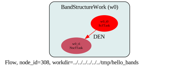
bandstructure_flow took care of creating the correct dependency between the two tasks. The NscfTask, indeed, depends on the ScfTask in w0/t0, whereas the ScfTask has no dependency:

flow.get_graphviz()

Note

Note that we have not used getden2 = -1 in the second dataset, since AbiPy knows how to connect the two Tasks. So there is no need for get* or ird* variables with AbiPy. Just specify the correct dependency and Python will do the rest!

To get useful information on the status of the flow, use:

flow.show_status()

Work #0: <BandStructureWork, node_id=309, workdir=../../../../../../tmp/hello_bands/w0>, Finalized=False 
+--------+-------------+---------+--------------+------------+----------+-----------------+--------+-----------+
| Task   | Status      | Queue   | MPI|Omp|Gb   | Warn|Com   | Class    | Sub|Rest|Corr   | Time   |   Node_ID |
+========+=============+=========+==============+============+==========+=================+========+===========+
| w0_t0  | Initialized | None    | 1|  1|2.0    | NA|NA      | ScfTask  | (0, 0, 0)       | None   |       310 |
+--------+-------------+---------+--------------+------------+----------+-----------------+--------+-----------+
| w0_t1  | Initialized | None    | 1|  1|2.0    | NA|NA      | NscfTask | (0, 0, 0)       | None   |       311 |
+--------+-------------+---------+--------------+------------+----------+-----------------+--------+-----------+

Meaning of the different columns:

• Task: short name of the task (usually w[index_of_work_in_flow]_t[index_of_task_in_work])

• Status: status of the task

• Queue: QueueName@Job identifier returned by the resource manager when the task is submitted

• (MPI|Omp|Gb): number of MPI procs, OMP threads, and memory per MPI proc

• (Warn|Com): number of Error/Warning/Comment messages found in the ABINIT log

• Class: the class of the Task

• (Sub|Rest|Corr): number of submissions/restarts/AbiPy corrections performed

• Node_ID: identifier of the task, used to select tasks or works in Python code or with abirun.py

Both Flow and Work are iterable. Iterating over a Flow gives Work objects, whereas iterating over a Work gives the Tasks inside that particular Work.

for work in flow:
    for task in work:
        print(task)

Flows and Works are containers, and we can select items in these containers with the syntax flow[start:stop] or work[start:stop]. This means that the previous loop is equivalent to the much more verbose version:

for i in range(len(flow)):
    work = flow[i]
    for t in range(len(work)):
        print(work[t])

At this point, it should not be difficult to understand that:

flow[0][0]

gives the first task in the first work of the flow, while

flow[-1][-1]

selects the last Task in the last Work. In several cases, we only need to iterate over a flat list of tasks without caring about the works. In this case, we can use:

for task in flow.iflat_tasks():
    print(task)

to iterate over all Tasks in the Flow.

How to build and run the Flow

The flow is still in memory and no file has been produced yet. To build the workflow, use:

if os.path.isdir("/tmp/hello_bands/"):
    import shutil
    shutil.rmtree("/tmp/hello_bands")

flow.build_and_pickle_dump()

0

This function creates the directories of the Flow:

(On macOS, the tree command might not be available. To fix this, see http://osxdaily.com/2016/09/09/view-folder-tree-terminal-mac-os-tree-equivalent/)

!tree /tmp/hello_bands

/tmp/hello_bands
├── __AbinitFlow__.pickle
├── _fix_flow.py
├── indata
├── outdata
├── tmpdata
└── w0
    ├── indata
    ├── outdata
    ├── t0
    │   ├── abipy_meta.json
    │   ├── indata
    │   ├── job.sh
    │   ├── outdata
    │   ├── run.abi
    │   └── tmpdata
    ├── t1
    │   ├── abipy_meta.json
    │   ├── indata
    │   ├── job.sh
    │   ├── outdata
    │   ├── run.abi
    │   └── tmpdata
    └── tmpdata

16 directories, 8 files

Let’s have a look at the files/directories associated with the first work (flow[0]):

flow[0].get_graphviz_dirtree()

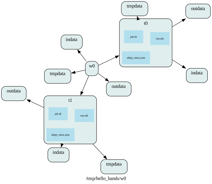
w0 is the directory containing the input files of the first work (well, we have only one work in our example). t0 and t1 contain the input files needed for the SCF and the NSCF run, respectively.

You might have noticed that all the Task directories have the same structure:

• run.abi: Input file

• run.files: Files file

• job.sh: Submission script

• outdata: Directory containing output data files

• indata: Directory containing input data files

• tmpdata: Directory with temporary files

Danger

AbinitFlow.pickle is the pickle file used to save the status of the Flow. Don’t touch it!

An Abinit Task has an AbinitInput, which in turn has a Structure:

 flow[0][0].input

##############################################
#### SECTION: basic
##############################################
ecut 6
nband 8
ngkpt 8 8 8
kptopt 1
nshiftk 1
shiftk 0 0 0
tolvrs 1e-06
##############################################
#### SECTION: files
##############################################
indata_prefix indata/in
tmpdata_prefix tmpdata/tmp
outdata_prefix outdata/out
pseudos /home/runner/work/abipy_book/abipy_book/abipy/abipy/data/pseudos/14si.pspnc
##############################################
#### STRUCTURE
##############################################
natom 2
ntypat 1
typat 1 1
znucl 14
xred
0.0000000000 0.0000000000 0.0000000000
0.2500000000 0.2500000000 0.2500000000
acell 1.0 1.0 1.0
rprim
6.3285005287 0.0000000000 3.6537614838
2.1095001762 5.9665675181 3.6537614838
0.0000000000 0.0000000000 7.3075229676

flow[0][0].input.structure

Structure Summary
Lattice
    abc : 3.86697462 3.86697462 3.86697462
 angles : 59.99999999999999 59.99999999999999 59.99999999999999
 volume : 40.88829179346891
      A : 3.3488982567096763 0.0 1.9334873100000005
      B : 1.1162994189032256 3.1573715557642927 1.9334873100000005
      C : 0.0 0.0 3.86697462
    pbc : True True True
PeriodicSite: Si1 (Si) (0.0, 0.0, 0.0) [0.0, 0.0, 0.0]
PeriodicSite: Si2 (Si) (1.116, 0.7893, 1.933) [0.25, 0.25, 0.25]

for p in flow[0][0].input.pseudos:
    print(p)

<NcAbinitPseudo: 14si.pspnc>
  summary: Troullier-Martins psp for element  Si        Thu Oct 27 17:31:21 EDT 1994
  number of valence electrons: 4.0
  maximum angular momentum: d
  angular momentum for local part: d
  XC correlation: LDA_XC_TETER93
  supports spin-orbit: False
  radius for non-linear core correction: 1.80626423934776
  hint for low accuracy: ecut: 0.0, pawecutdg: 0.0
  hint for normal accuracy: ecut: 0.0, pawecutdg: 0.0
  hint for high accuracy: ecut: 0.0, pawecutdg: 0.0

Let’s print the value of kptopt for all the tasks in our flow with:

print([task.input["kptopt"] for task in flow.iflat_tasks()])

[1, -2]

which, in this particular case, gives the same result as:

print([task.input["kptopt"] for task in flow[0]])

[1, -2]

Executing a Flow

The Flow can be executed with two different approaches: a programmatic interface based on flow.make_scheduler, or the abirun.py script. In this section, we discuss the first approach because it plays well with Jupyter notebooks. Note, however, that abirun.py is highly recommended, especially when running non-trivial calculations.

flow.make_scheduler().start()

Using scheduler v >= 3.0.0

[Wed Sep 30 16:02:58 2026] Number of launches: 1

Work #0: <BandStructureWork, node_id=309, workdir=../../../../../../tmp/hello_bands/w0>, Finalized=False 
+--------+-------------+------------+--------------+------------+----------+-----------------+----------+-----------+
| Task   | Status      | Queue      | MPI|Omp|Gb   | Warn|Com   | Class    | Sub|Rest|Corr   | Time     |   Node_ID |
+========+=============+============+==============+============+==========+=================+==========+===========+
| w0_t0  | Submitted   | 4453@githu | 2|  1|2.0    | NA|NA      | ScfTask  | (1, 0, 0)       | 0:00:00Q |       310 |
+--------+-------------+------------+--------------+------------+----------+-----------------+----------+-----------+
| w0_t1  | Initialized | None       | 1|  1|2.0    | NA|NA      | NscfTask | (0, 0, 0)       | None     |       311 |
+--------+-------------+------------+--------------+------------+----------+-----------------+----------+-----------+

nbdbuf is not specified in input, using `nbdbuf = 2 * nspinor` that may be too small!"
As a consequence, the NSCF cycle may have problems to converge the last bands within nstep iterations.
To avoid this problem specify nbdbuf in the input file and adjust nband accordingly.

[Wed Sep 30 16:03:03 2026] Number of launches: 1

Work #0: <BandStructureWork, node_id=309, workdir=../../../../../../tmp/hello_bands/w0>, Finalized=False 
+--------+-----------+------------+--------------+------------+----------+-----------------+----------+-----------+
| Task   | Status    | Queue      | MPI|Omp|Gb   | Warn|Com   | Class    | Sub|Rest|Corr   | Time     |   Node_ID |
+========+===========+============+==============+============+==========+=================+==========+===========+
| w0_t0  | Completed | 4453@githu | 2|  1|2.0    | 2|  2      | ScfTask  | (1, 0, 0)       | 0:00:01R |       310 |
+--------+-----------+------------+--------------+------------+----------+-----------------+----------+-----------+
| w0_t1  | Submitted | 4472@githu | 2|  1|2.0    | NA|NA      | NscfTask | (1, 0, 0)       | 0:00:00Q |       311 |
+--------+-----------+------------+--------------+------------+----------+-----------------+----------+-----------+

Work #0: <BandStructureWork, node_id=309, workdir=../../../../../../tmp/hello_bands/w0>, Finalized=True 
  Finalized works are not shown. Use verbose > 0 to force output.

all_ok reached

Calling flow.finalize() ...

Submitted on: Wed Sep 30 16:02:57 2026
Completed on: Wed Sep 30 16:03:07 2026
Elapsed time: 0:00:10.008639
Flow completed successfully

0

The flow keeps track of the different actions performed by the Python code:

flow.show_history()

================================================================================
 <BandStructureWork, node_id=309, workdir=../../../../../../tmp/hello_bands/w0> 
================================================================================
[Wed Sep 30 16:03:02 2026] In on_ok with sender <ScfTask, node_id=310, workdir=../../../../../../tmp/hello_bands/w0/t0>
[Wed Sep 30 16:03:07 2026] In on_ok with sender <NscfTask, node_id=311, workdir=../../../../../../tmp/hello_bands/w0/t1>
[Wed Sep 30 16:03:07 2026] Finalized set to True
[Wed Sep 30 16:03:07 2026] Work <BandStructureWork, node_id=309, workdir=../../../../../../tmp/hello_bands/w0> is finalized and broadcasts signal S_OK
[Wed Sep 30 16:03:07 2026] Node <BandStructureWork, node_id=309, workdir=../../../../../../tmp/hello_bands/w0> broadcasts signal Completed

===============================================================================
=== <ScfTask, node_id=310, workdir=../../../../../../tmp/hello_bands/w0/t0> ===
===============================================================================
[Wed Sep 30 16:02:57 2026] Status changed to Ready. msg: Status set to Ready
[Wed Sep 30 16:02:57 2026] Setting input variables: {'autoparal': 1, 'max_ncpus': 2, 'mem_test': 0, 'chkparal': 0}
[Wed Sep 30 16:02:57 2026] Old values: {'autoparal': None, 'max_ncpus': None, 'mem_test': None, 'chkparal': None}
[Wed Sep 30 16:02:58 2026] Setting input variables: {'npimage': 1, 'npkpt': 2, 'npspinor': 1, 'npfft': 1, 'npband': 1, 'bandpp': 1}
[Wed Sep 30 16:02:58 2026] Old values: {'npimage': None, 'npkpt': None, 'npspinor': None, 'npfft': None, 'npband': None, 'bandpp': None}
[Wed Sep 30 16:02:58 2026] Status changed to Initialized. msg: finished autoparal run
[Wed Sep 30 16:02:58 2026] Submitted with MPI=2, Omp=1, Memproc=2.0 [GB] Submitted to queue 
[Wed Sep 30 16:03:02 2026] Task completed status set to OK based on abiout
[Wed Sep 30 16:03:02 2026] Finalized set to True
[Wed Sep 30 16:03:02 2026] Node <ScfTask, node_id=310, workdir=../../../../../../tmp/hello_bands/w0/t0> broadcasts signal Completed

================================================================================
=== <NscfTask, node_id=311, workdir=../../../../../../tmp/hello_bands/w0/t1> ===
================================================================================
[Wed Sep 30 16:03:02 2026] Status changed to Ready. msg: Status set to Ready
[Wed Sep 30 16:03:02 2026] Need path `/tmp/hello_bands/w0/t0/outdata/out_DEN` with extension: `DEN`
[Wed Sep 30 16:03:02 2026] Linking path /tmp/hello_bands/w0/t0/outdata/out_DEN --> /tmp/hello_bands/w0/t1/indata/in_DEN
[Wed Sep 30 16:03:02 2026] 
nbdbuf is not specified in input, using `nbdbuf = 2 * nspinor` that may be too small!"
As a consequence, the NSCF cycle may have problems to converge the last bands within nstep iterations.
To avoid this problem specify nbdbuf in the input file and adjust nband accordingly.

[Wed Sep 30 16:03:02 2026] Setting input variables: {'ngfft': array([18, 18, 18])}
[Wed Sep 30 16:03:02 2026] Old values: {'ngfft': None}
[Wed Sep 30 16:03:02 2026] Adding connecting vars {'irdden': 1}
[Wed Sep 30 16:03:02 2026] Setting input variables: {'irdden': 1}
[Wed Sep 30 16:03:02 2026] Old values: {'irdden': None}
[Wed Sep 30 16:03:02 2026] Setting input variables: {'autoparal': 1, 'max_ncpus': 2, 'mem_test': 0, 'chkparal': 0}
[Wed Sep 30 16:03:02 2026] Old values: {'autoparal': None, 'max_ncpus': None, 'mem_test': None, 'chkparal': None}
[Wed Sep 30 16:03:03 2026] Setting input variables: {'npimage': 1, 'npkpt': 2, 'npspinor': 1, 'npfft': 1, 'npband': 1, 'bandpp': 1}
[Wed Sep 30 16:03:03 2026] Old values: {'npimage': None, 'npkpt': None, 'npspinor': None, 'npfft': None, 'npband': None, 'bandpp': None}
[Wed Sep 30 16:03:03 2026] Status changed to Initialized. msg: finished autoparal run
[Wed Sep 30 16:03:03 2026] Submitted with MPI=2, Omp=1, Memproc=2.0 [GB] Submitted to queue 
[Wed Sep 30 16:03:07 2026] Task completed status set to OK based on abiout
[Wed Sep 30 16:03:07 2026] Finalized set to True
[Wed Sep 30 16:03:07 2026] Node <NscfTask, node_id=311, workdir=../../../../../../tmp/hello_bands/w0/t1> broadcasts signal Completed

================================================================================
======== <Flow, node_id=308, workdir=../../../../../../tmp/hello_bands> ========
================================================================================
[Wed Sep 30 16:03:07 2026] Calling flow.finalize.
[Wed Sep 30 16:03:07 2026] Finalized set to True

stty: 'standard input': Inappropriate ioctl for device

If you read the logs carefully, you will realize that in the first iteration of the scheduler, only the ScfTask is executed, because the second task depends on it. After the initial submission, the scheduler starts to monitor all the tasks in the flow.

When the ScfTask completes, the dependency of the NscfTask is fulfilled and a new submission takes place. Once the second task completes, the scheduler calls flow.finalize to execute (optional) logic that performs some sort of cleanup or post-processing. At this point, all the tasks in the flow are completed and the scheduler exits.

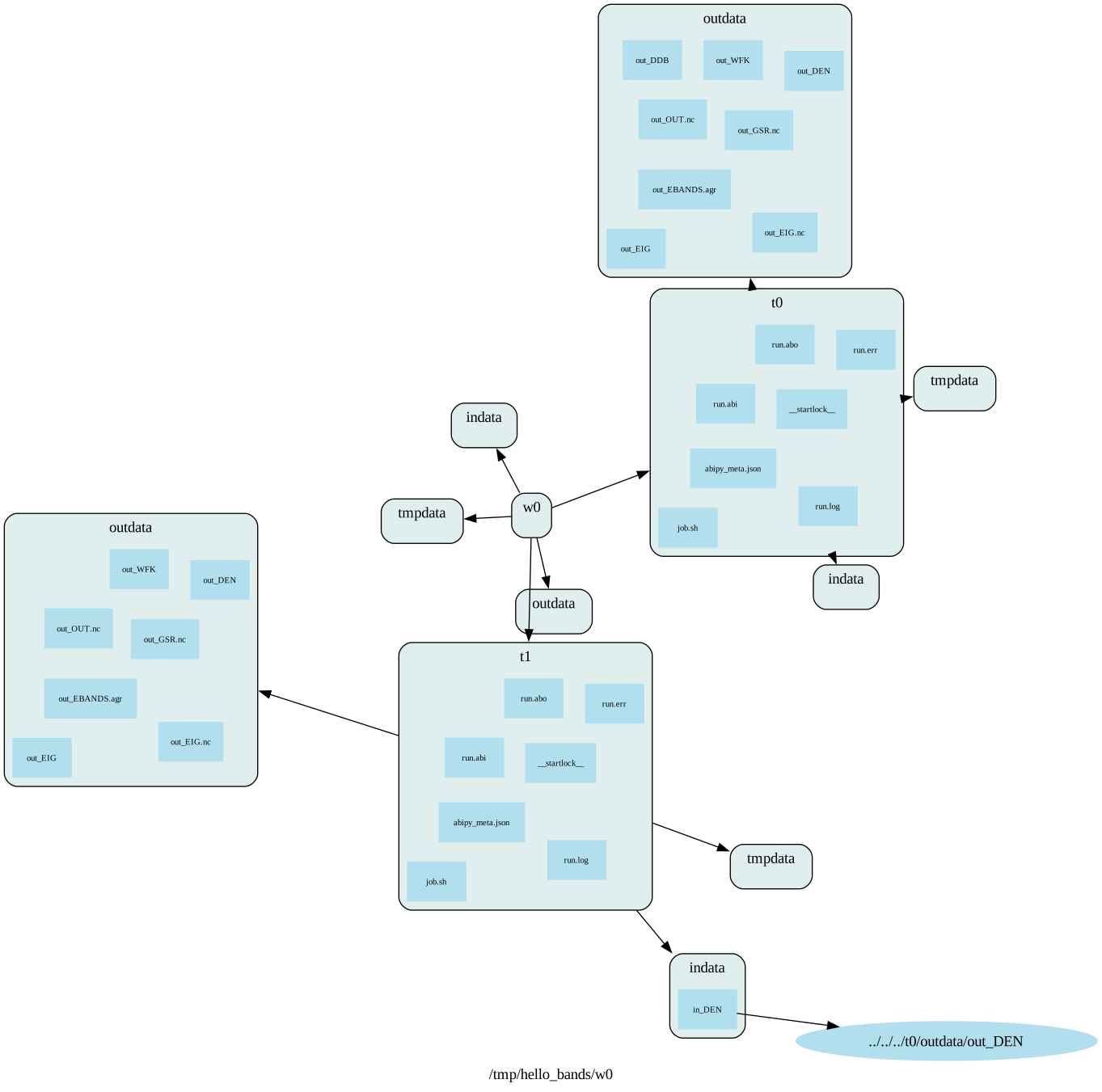
Now we can have a look at the different output files produced by the flow with:

flow[0].get_graphviz_dirtree()

or list only the files with a given extension:

flow.listext("GSR.nc")

Found 2 files with extension `GSR.nc` produced by the flow
File                                                          Size [Mb]    Node_ID  Node Class
----------------------------------------------------------  -----------  ---------  ------------
../../../../../../tmp/hello_bands/w0/t0/outdata/out_GSR.nc         9.63        310  ScfTask
../../../../../../tmp/hello_bands/w0/t1/outdata/out_GSR.nc         9.62        311  NscfTask

The nice thing about the flow is that it knows how to locate and interpret the different input/output files produced by Abinit. As a consequence, it is very easy to expose the AbiPy post-processing tools through an easy-to-use API that only requires tasks/works/flows plus very few input arguments.

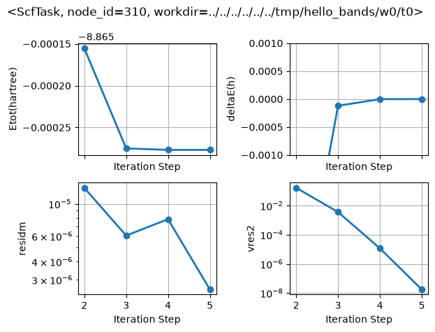
Let’s call, for instance, the inspect method to plot the self-consistent cycles:

flow.inspect(tight_layout=True);

Task <NscfTask, node_id=311, workdir=../../../../../../tmp/hello_bands/w0/t1> does not provide an inspect method

In the other AbiPy tutorials, we have explained how to use abiopen to create Python objects from netcdf files. Well, the same code can be reused with the flow: it is just a matter of replacing

with abiopen(filepath) as gsr:

with

with task.open_gsr() as gsr:

Note that there is no need to specify the file path when you use the task-based API, because the Task knows how to locate its GSR.nc output. Let’s practice a bit:

with flow[0][0].open_gsr() as gsr:
    ebands_kmesh = gsr.ebands

with flow[0][1].open_gsr() as gsr:
    gsr.ebands.plotly_with_edos(ebands_kmesh.get_edos(), with_gaps=True);

More on Works, Tasks and dependencies

In the previous example, we constructed a workflow for band structure calculations starting from two input files and the magic line

flow = flowtk.bandstructure_flow(workdir, scf_input, nscf_input)

Now it is time to explain in more detail the syntax and the API used in AbiPy to build a flow with dependencies. Let’s build a Flow from scratch and use graphviz after each step to show what’s happening. We start with an empty flow in the hello_flow directory:

hello_flow = flowtk.Flow(workdir="hello_flow")
hello_flow.get_graphviz()

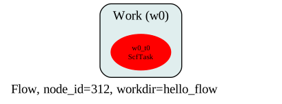
Now we add a new Task by simply passing an AbinitInput for an SCF calculation:

hello_flow.register_scf_task(scf_input, append=True)
hello_flow.get_graphviz()

Now the tricky part. We want to register an NSCF calculation that depends on the scf_task in w0_t0 via the DEN file. We can use the same API, but we must specify the dependency between the two steps with the {scf_task: "DEN"} dictionary:

hello_flow.register_nscf_task(nscf_input, deps={hello_flow[0][0]: "DEN"}, append=True)
hello_flow.get_graphviz(engine="dot")

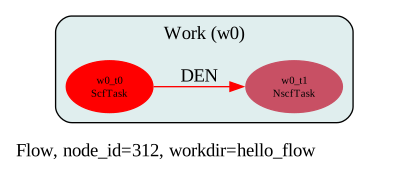
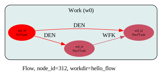
Excellent, we managed to build our first AbiPy flow with inter-dependent tasks in just six lines of code (including the three calls to graphviz). Now let’s assume we want to add a second NSCF calculation (NscfTask) in which we change one of the input parameters, e.g. the number of bands, and that, for some reason, we really want to reuse the output WFK file produced by w0_t1 to initialize the eigenvalue solver (obviously, we still need a DEN file). How can we express this with AbiPy?

Well, the syntax for the new dependencies is just:

deps = {hello_flow[0][0]: "DEN", hello_flow[0][1]: "WFK"}

but we should also change the input variable nband in nscf_input before creating the new NscfTask (remember that building a Task requires an AbinitInput object and a list of dependencies, if any).

Now, there are two ways to increase nband: the wrong way and the correct one! Let’s start with the wrong way, because it’s always useful to learn from our mistakes. Let’s print some values just for the record:

t1 = flow[0][1]
print("nband in the first NscfTask:", t1.input["nband"])

nband in the first NscfTask: 8

Now let’s use the “recipe” recommended to us by the FORTRAN guru of our group:

# Just copy the previous input and change nband, it's super-easy, the FORTRAN guru said!
new_input = t1.input
new_input["nband"] = 1000

print("nband in the first NscfTask:", t1.input["nband"])
print("nband in the new input:", new_input["nband"])

nband in the first NscfTask: 1000
nband in the new input: 1000

Tada! Thanks to the trick of our beloved FORTRAN guru, we ended up with two inputs with the same number of bands (1000!). Why?

Because AbinitInput is implemented internally with a dictionary, Python dictionaries are mutable, and Python variables are essentially references (they do not store the data, but the address of the data).

a = {"foo": "bar"}
b = a
c = a.copy()
a["hello"] = "world"
print("a dict:", a)
print("b dict:", b)
print("c dict:", c)

a dict: {'foo': 'bar', 'hello': 'world'}
b dict: {'foo': 'bar', 'hello': 'world'}
c dict: {'foo': 'bar'}

For a more technical explanation, see here.

To avoid this mistake, we need to copy the object before changing it:

t1.input["nband"] = 8 # back to the old value

new_input = t1.input.new_with_vars(nband=1000)  # Copy and change nband

print("nband in the first NscfTask:", t1.input["nband"])
print("nband in the new input:", new_input["nband"])

nband in the first NscfTask: 8
nband in the new input: 1000

Now we can finally add the second NscfTask with 1000 bands:

hello_flow.register_nscf_task(new_input, deps={hello_flow[0][0]: "DEN", hello_flow[0][1]: "WFK"}, append=True)
hello_flow.get_graphviz(engine="dot")

print([task.input["nband"] for task in hello_flow.iflat_tasks()])

[8, 8, 1000]

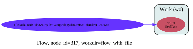
Note that AbiPy dependencies can also be fulfilled with external files that are already available when the flow is constructed. The syntax is the same as before: it is just a matter of using the absolute path to the DEN file as key of the dictionary instead of a Task. Let’s start with a new Flow to avoid confusion, and create an NscfTask that starts from a pre-computed DEN file:

flow_with_file = flowtk.Flow(workdir="flow_with_file")

den_filepath = abidata.ref_file("si_DEN.nc")
flow_with_file.register_nscf_task(nscf_input, deps={den_filepath: "DEN"})

flow_with_file.get_graphviz(engine="dot")

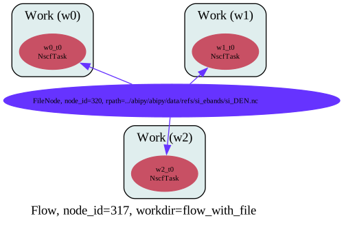
A call to new_with_vars inside a Python for loop is all we need to add two more NscfTasks with different nband, all starting from the same DEN file:

for nband in [10, 20]:
    flow_with_file.register_nscf_task(nscf_input.new_with_vars(nband=nband),
                                      deps={den_filepath: "DEN"}, append=False)

print([task.input["nband"] for task in flow_with_file.iflat_tasks()])
flow_with_file.get_graphviz()

[8, 10, 20]

At this point, you may ask why we need Works since all the examples presented so far mainly involve the Flow object.

The answer is that Works allow us to encapsulate reusable logic in magic boxes that can perform a lot of useful work. These boxes can then be connected together to generate more complicated workflows. We have already encountered the BandStructureWork at the beginning of this lesson, and now it is time to introduce another fancy animal of the AbiPy zoo: the PhononWork.

abilab.print_doc(flowtk.PhononWork)

class PhononWork(Work, MergeDdb):
    """
    This work consists of nirred Phonon tasks where nirred is
    the number of irreducible atomic perturbations for a given set of q-points.
    It provides the callback method (on_all_ok) that calls mrgddb and mrgdv to merge
    all the partial DDB (POT) files produced.
    The two files are available in the output directory of the Work.

    .. rubric:: Inheritance Diagram
    .. inheritance-diagram:: PhononWork
    """

abilab.print_doc(flowtk.PhononWork.from_scf_task)

    @classmethod
    def from_scf_task(
        cls,
        scf_task: ScfTask,
        qpoints,
        is_ngqpt=False,
        with_becs=False,
        with_quad=False,
        with_flexoe=False,
        with_dvdb=True,
        tolerance=None,
        ddk_tolerance=None,
        ndivsm=0,
        qptopt=1,
        prtwf=-1,
        prepgkk=0,
        manager=None,
    ) -> PhononWork:
        """
        Construct a `PhononWork` from a |ScfTask| object.
        The input file for phonons is automatically generated from the input of the ScfTask.
        Each phonon task depends on the WFK file produced by the `scf_task`.

        Args:
            scf_task: |ScfTask| object.
            qpoints: q-points in reduced coordinates. Accepts single q-point, list of q-points
                or three integers defining the q-mesh if `is_ngqpt`.
            is_ngqpt: True if `qpoints` should be interpreted as divisions instead of q-points.
            with_becs: Activate calculation of Electric field and Born effective charges.
            with_quad: Activate calculation of dynamical quadrupoles. Require `with_becs`
                Note that only selected features are compatible with dynamical quadrupoles.
                Please consult <https://docs.abinit.org/topics/longwave/>
            with_flexoe: True to activate computation of flexoelectric tensor. Require `with_becs`
            with_dvdb: True to merge POT1 files associated to atomic perturbations in the DVDB file
                at the end of the calculation
            tolerance: dict {"varname": value} with the tolerance to be used in the phonon run.
                None to use AbiPy default.
            ddk_tolerance: dict {"varname": value} with the tolerance used in the DDK run if with_becs.
                None to use AbiPy default.
            ndivsm: If different from zero, activate computation of electron band structure.
                if > 0, it's the number of divisions for the smallest segment of the path (Abinit variable).
                if < 0, it's interpreted as the pymatgen `line_density` parameter in which the number of points
                in the segment is proportional to its length. Typical value: -20.
                This option is the recommended one if the k-path contains two high symmetry k-points that are very close
                as ndivsm > 0 may produce a very large number of wavevectors.
                if 0, deactivate band structure calculation.
            qptopt: Option for the generation of q-points. Default: 1 i.e. use msym spatial symmetries + TR.
            prtwf: Controls the output of the first-order WFK.
                By default we set it to -1 when q != 0 so that AbiPy is still able
                to restart the DFPT task if the calculation is not converged (worst case scenario)
                but we avoid the output of the 1-st order WFK if the calculation converged successfully.
                Non-linear DFPT tasks should not be affected since they assume q == 0.
            prepgkk: option to compute only the irreducible preturbations or all perturbations
                for the chosen set of q-point. Default: 0 (irred. pret. only)
            manager: |TaskManager| object.
        """

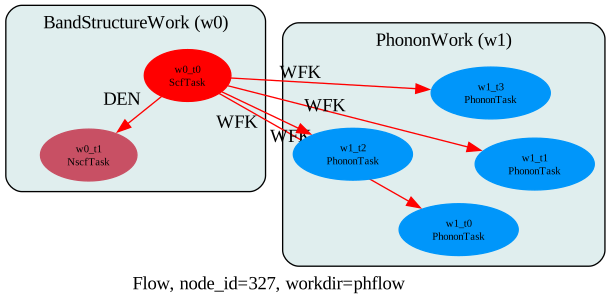
The docstring suggests that, given an scf_task, I can construct a magic box to compute phonons. But wait, I already have such a task! Actually, I already have another magic box to compute the electronic band structure, and it would be really great if I could compute the electronic and vibrational properties in a single flow. Let’s connect the two boxes together with:

# Create new flow.
ph_flow = flowtk.Flow(workdir="phflow")

# Band structure (SCF + NSCF)
bands_work = flowtk.BandStructureWork(scf_input, nscf_input, dos_inputs=None)
ph_flow.register_work(bands_work)

# Build second work from scf_task.
scf_task = bands_work[0]
ph_work = flowtk.PhononWork.from_scf_task(scf_task, [2, 2, 2], is_ngqpt=True, tolerance=None)
ph_flow.register_work(ph_work)

ph_flow.get_graphviz()

Now, it turns out that the PhononWork merges all the DDB files produced by its PhononTasks and puts the final output file in its outdir. So, from the AbiPy perspective, a PhononWork is not that different from an ScfTask that produces e.g. a DEN file. This means that we can connect other magic boxes to our PhononWork, e.g. a set of EPhTasks that require a DDB file and another input file with the DFPT potentials (the DVDB, which PhononWork merges similarly to what is done for the DDB).

# EPH tasks require 3 input files (WFK, DDB, DVDB)
eph_deps = {ph_flow[0][1]: "WFK", ph_work: ["DDB", "DVDB"]}

for i, ecut in enumerate([2, 3, 4]):
    ph_flow.register_eph_task(nscf_input.new_with_vars(ecut=ecut), deps=eph_deps, append=(i != 0))

ph_flow.get_graphviz()

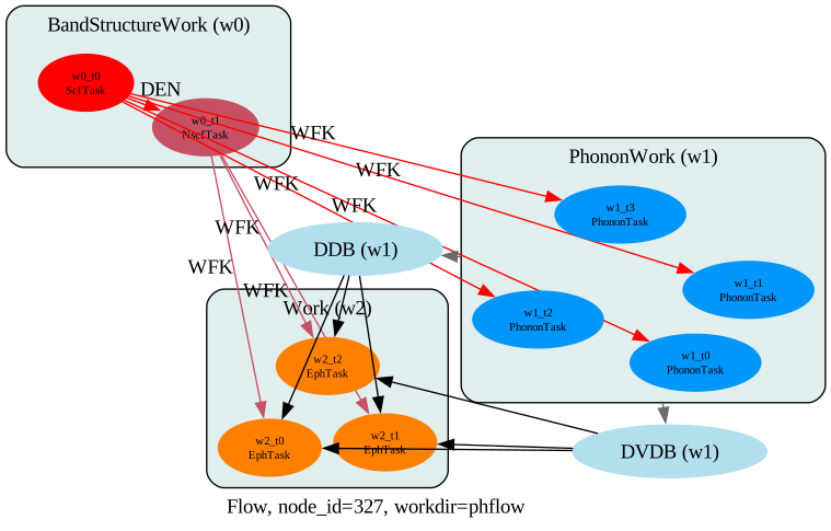
This explains why AbiPy uses this classification in terms of Tasks/Works/Flows: we can implement highly specialized Works/Tasks to solve specific problems and then connect all these nodes together. Just 11 lines of code to get electrons + phonons + (electrons + phonons)!

But wait, did you see the gorilla?

from IPython.display import YouTubeVideo
YouTubeVideo("vJG698U2Mvo")

There’s indeed a bug in the last step. The connections among the nodes are OK, but we made a mistake while creating the EPhTasks with:

ph_flow.register_eph_task(nscf_input.new_with_vars(ecut=ecut), ...)

because we passed an input for a standard band structure calculation to something that is supposed to deal with the E-PH interaction. This example stresses that the AbiPy Flow, by design, does not try to validate your input to make sure it is consistent with the workflow logic. This is done on purpose, for two reasons:

• Expert users should be able to customize/tune their input files, and validating all the possible cases in Python is not trivial.

• Only Abinit (and God) knows at run time whether your input file makes sense, and we can’t reimplement the same logic in Python.

At this point, you may wonder why we have so many different AbiPy Tasks (ScfTask, NscfTask, RelaxTask, PhononTask, EPHTask, …) if there’s no input validation when we create them.

The answer is that we need all these subclasses to implement extra logic that is specific to each particular calculation. AbiPy, indeed, does not just submit jobs: it also monitors the evolution of the calculation and executes predefined code to fix run-time problems (and these problems are calculation-specific). An example will help clarify this point.

Restarting jobs is one of the typical problems encountered in ab-initio calculations, and restarting a RelaxTask requires a different logic from e.g. restarting an ScfTask. For an ScfTask, we only need to use the output WFK (DEN) of the previous execution as input of the restarted job, while a RelaxTask must also reuse the (unconverged) final structure of the previous job to be effective and avoid a possibly infinite loop. In a nutshell, when you use a particular Task/Work class, you are telling AbiPy how to handle possible problems at run time, and you are also specifying the actions that should be performed at the beginning/end of the execution.

Abirun.py

Executing

flow.make_scheduler().start()

inside a Jupyter notebook is handy if you are dealing with small calculations that take a few seconds or minutes. This approach, however, is impractical for large flows or big calculations requiring hours or days, even on massively parallel machines. In this case, one would like to run the scheduler in a separate process in the background, so that the scheduler is not killed when the Jupyter server is closed.

To start the scheduler in a separate process, use the abirun.py script. The syntax is:

abirun.py flow_workdir COMMAND

where flow_workdir is the directory containing the Flow (the directory with the pickle file) and COMMAND selects the operation to be performed.

Typical examples:

abirun.py /tmp/hello_bands status

checks the status of the Flow and prints the results to screen, while

nohup abirun.py /tmp/hello_bands scheduler > sched.log 2> sched.err &

starts the scheduler in the background, redirecting the standard output to the sched.log file.

Important

nohup is a standard Unix tool. The command makes the scheduler immune to hangups, so that you can close the shell session without killing the scheduler.

This brings us to the last and most crucial question: how do we configure AbiPy to run Abinit workflows on different architectures, ranging from standard laptops to high-performance supercomputers?

Unfortunately, this notebook is already quite long, and these details are best covered in the technical documentation. What should be stressed here is that the behaviour can be customized with two YAML files. All the information related to your environment (Abinit build, modules, resource managers, shell environment) is read from the manager.yml configuration file, which is usually located in the ~/.abinit/abipy/ directory. The options for the Python scheduler responsible for job submission are given in scheduler.yml.

For a more complete description of these configuration options, please consult the TaskManager documentation. A list of configuration files for different machines and clusters is available here, while the Flows HOWTO gathers answers to frequently asked questions.

Last but not least, check out our gallery of AbiPy Flows for inspiration.