Lobster output files#
This example shows how to analyze the output files produced by Lobster
Use
abiopen.py FILE
with the --expose or --print for a command line interface
and --notebook to generate a jupyter notebook from a lobster FILE.
Note: The code in this notebook requires abipy >= 0.6
Let’s start by importing the basic modules needed for this tutorial.
import warnings
warnings.filterwarnings("ignore")  # Ignore warnings

from abipy import abilab
abilab.enable_notebook() # This line tells AbiPy we are running inside a notebook
import abipy.data as abidata

# This line configures matplotlib to show figures embedded in the notebook.
# Replace `inline` with `notebook` in classic notebook
%matplotlib inline

# Option available in jupyterlab. See https://github.com/matplotlib/jupyter-matplotlib
#%matplotlib widget
How to analyze the COHPCAR file#
# Path to one of the reference file shipped with AbiPy
import os
dirpath = os.path.join(abidata.dirpath, "refs", "lobster_gaas")
filename = os.path.join(dirpath, "GaAs_COHPCAR.lobster.gz")

# Open the COHPCAR.lobster file (same API for COOPCAR.lobster)
cohp_file = abilab.abiopen(filename)
print(cohp_file)
Creating temporary file: /tmp/tmpbt4qs_hsGaAs_COHPCAR.lobster

COHP: Number of energies: 401, from -14.035 to 6.015 (eV) with E_fermi set 0 (was 2.298)
has_partial_projections: True, nsppol: 1
Number of pairs: 2
[0] Ga@0 --> As@1
[1] As@1 --> Ga@0
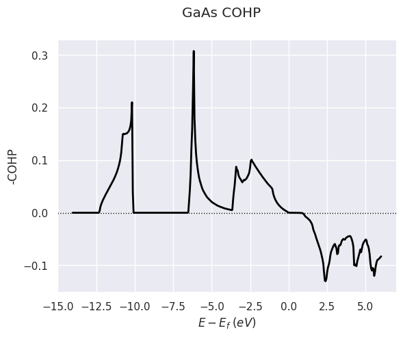
To plot the COHP averaged over all atom pairs specified:
cohp_file.plot(title="GaAs COHP");
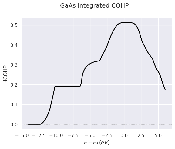
To plot the integrated COHP averaged over all atom pairs:
cohp_file.plot(what="i", title="GaAs integrated COHP");
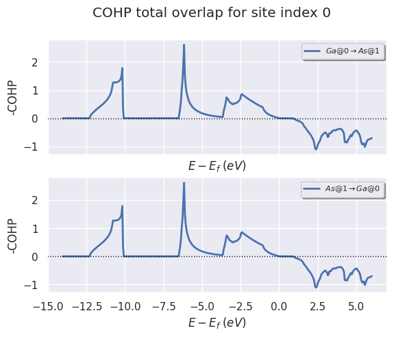
To plot the total overlap for all sites listed in from_site_index
cohp_file.plot_site_pairs_total(from_site_index=[0, 1], title="COHP total overlap for site index 0");
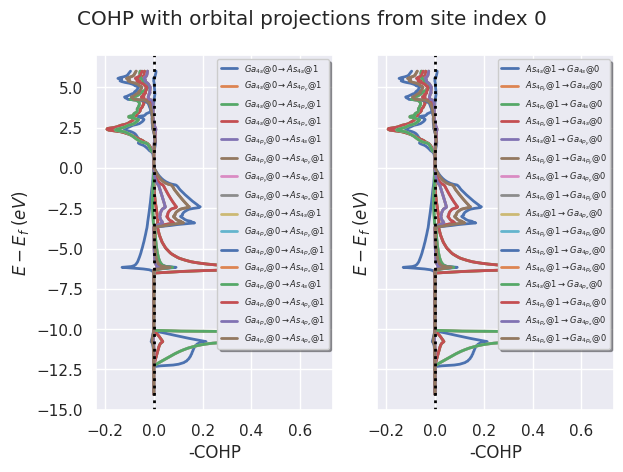
To plot partial crystal orbital projections for all sites listed in from_site_index:
cohp_file.plot_site_pairs_partial(from_site_index=[0, 1],
                                  title="COHP with orbital projections from site index 0",
                                  fontsize=6, tight_layout=True);
#cohp_file.plot_average_pairs(with_site_index=[0]);
Use abiopen to open the MDF:
How to analyze the ICOHPLIST file#
# Path to one of the AbiPy file
dirpath = os.path.join(abidata.dirpath, "refs", "lobster_gaas")
filename = os.path.join(dirpath, "GaAs_ICOHPLIST.lobster.gz")

# Open the ICOHPCAR.lobster file.
icohp_file = abilab.abiopen(filename)
print(icohp_file)
Creating temporary file: /tmp/tmp2y8n10irGaAs_ICOHPLIST.lobster
Number of pairs: 2
 index0  index1 type0 type1  spin  average distance n_bonds   pair
      0       1    Ga    As     0 -4.36062  2.49546    None (0, 1)
      1       0    As    Ga     0 -4.36062  2.49546    None (1, 0)
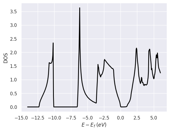
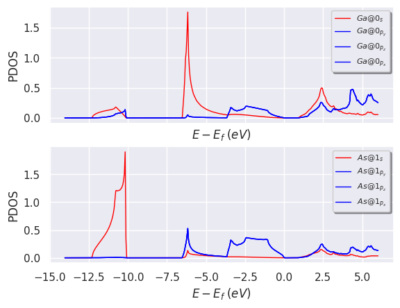
How to analyze the DOSCAR file#
dirpath = os.path.join(abidata.dirpath, "refs", "lobster_gaas")
filename = os.path.join(dirpath, "GaAs_DOSCAR.lobster.gz")

# Open the ICOHPCAR.lobster file.
doscar = abilab.abiopen(filename)
print(doscar)
Creating temporary file: /tmp/tmpxn7e6d9uGaAs_DOSCAR.lobster
Number of energies: 401, from -14.035 to 6.015 (eV) with E_fermi set to 0 (was 2.298)
nsppol: 1
Number of sites in projected DOS: 2
0 --> {4s, 4p_y, 4p_z, 4p_x}
1 --> {4s, 4p_y, 4p_z, 4p_x}
doscar.plot();
doscar.plot_pdos_site(site_index=[0, 1]);
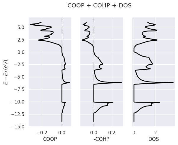
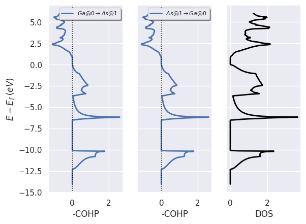
Analyzing all Lobster output files with LobsterAnalyzer#
Let’s assume we have a directory with lobster output files
for COOP, COHP, DOS and we need to produce plots showing all these results altogether.
In this case, one can use the LobsterAnalyzer object and initialize it from the directory
containing the output files.
dirpath = os.path.join(abidata.dirpath, "refs", "lobster_gaas")

# Open the all the lobster files produced in directory dirpath
# with the (optional) prefix GaAs_
lobana = abilab.LobsterAnalyzer.from_dir(dirpath, prefix="GaAs_")
print(lobana.to_string(verbose=1))
================================= COOP File =================================
Name: GaAs_COOPCAR.lobster.gz
Directory: /home/runner/work/abipy_book/abipy_book/abipy/abipy/data/refs/lobster_gaas
Size: 23.04 kB
Access Time: Thu Jan 15 12:19:59 2026
Modification Time: Thu Jan 15 12:15:09 2026
Change Time: Thu Jan 15 12:15:09 2026

COOP: Number of energies: 401, from -14.035 to 6.015 (eV) with E_fermi set 0 (was 2.298)
has_partial_projections: True, nsppol: 1
Number of pairs: 2
[0] Ga@0 --> As@1
[1] As@1 --> Ga@0

================================= COHP File =================================
Name: GaAs_COHPCAR.lobster.gz
Directory: /home/runner/work/abipy_book/abipy_book/abipy/abipy/data/refs/lobster_gaas
Size: 24.06 kB
Access Time: Thu Jan 15 12:19:57 2026
Modification Time: Thu Jan 15 12:15:09 2026
Change Time: Thu Jan 15 12:15:09 2026

COHP: Number of energies: 401, from -14.035 to 6.015 (eV) with E_fermi set 0 (was 2.298)
has_partial_projections: True, nsppol: 1
Number of pairs: 2
[0] Ga@0 --> As@1
[1] As@1 --> Ga@0

============================== ICHOHPLIST File ==============================
Number of pairs: 2
 index0  index1 type0 type1  spin  average distance n_bonds   pair
      0       1    Ga    As     0 -4.36062  2.49546    None (0, 1)
      1       0    As    Ga     0 -4.36062  2.49546    None (1, 0)

=============================== Lobster DOSCAR ===============================
Number of energies: 401, from -14.035 to 6.015 (eV) with E_fermi set to 0 (was 2.298)
nsppol: 1
Number of sites in projected DOS: 2
0 --> {4s, 4p_y, 4p_z, 4p_x}
1 --> {4s, 4p_y, 4p_z, 4p_x}
To plot COOP + COHP + DOS, use:
lobana.plot(title="COOP + COHP + DOS");
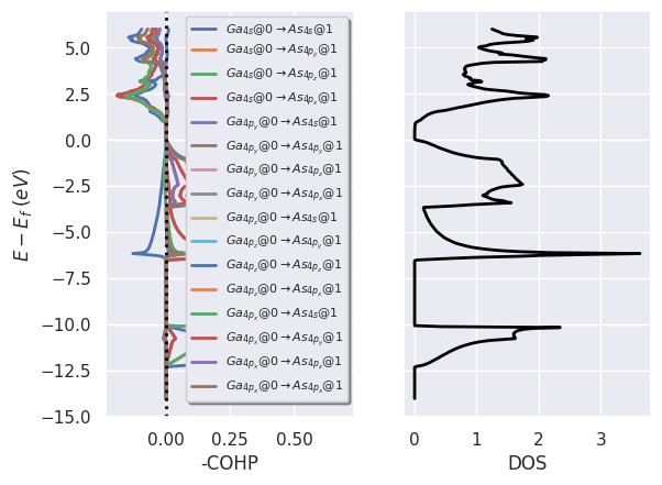
To plot COHP for all sites in from_site_index and Lobster DOS:
lobana.plot_coxp_with_dos(from_site_index=[0, 1]);
# Plot orbital projections.
lobana.plot_coxp_with_dos(from_site_index=[0], with_orbitals=True);
#lobana.plot_with_ebands(ebands="out_GSR.nc")