\(G_0W_0\) band structure with star-function interpolation#
Standard functionals such as LDA or GGA, systematically underestimate band gaps, giving values that are about 30-40% smaller than experimental data. The inability of standard Kohn-Sham (KS) theory to give band gaps close to experiment is often referred to as the band-gap problem.
From a theoretical point of view this is not surprising since KS eigenvalues are not supposed to give the correct band energies. The band structure of a crystal is rigorously defined as the energies needed to add or subtract electrons from the many-body system which, in turn, are related to the difference between total energies of many-body states differing by one electron.
An alternative, more traditional, approach to the study of exchange-correlation effects in many-body systems is provided by Many-Body Perturbation Theory (MBPT) which defines a rigorous approach to the description of excited-state properties, based on the Green’s function formalism. In this lesson, we discuss how to use the MBPT part of ABINIT to compute the band-structure of silicon within the so-called \(G_0W_0\) approximation. For a very brief introduction to the many-body formalism, please consult the MBPT_notes
Description of the lesson#
In this lesson, we construct an AbiPy flow made of two works. The first work is a standard KS band-structure calculation consisting of an initial GS calculation to get the density, followed by two NSCF calculations. The first NSCF task computes the KS eigenvalues on a high-symmetry path in the BZ, whereas the second NSCF task employs a homogeneous k-mesh so that one can compute the DOS from the KS eigenvalues.
The second work represents the real GW workflow that uses the density computed in the first task of the previous work to compute the KS bands for many empty states. The WFK file produced in this step is then used to compute the screened interaction \(W\). Finally, we perform a self-energy calculation that uses the \(W\) produced in the previous step and the WFK file to compute the matrix elements of the self-energy and the \(G_0W_0\) corrections for all the k-points in the IBZ and 8 bands (4 occupied + 4 empty). Once the flow is completed, we can interpolate the \(G_0W_0\) corrections.
Do not worry if there are steps of the entire procedure that are not clear to you. \(GW\) calculations are much more complicated than standard KS band structures and the main goal of this lesson is to give you an overview of the Abipy capabilities.
Let’s start with the usual import section:
import numpy as np
import warnings
warnings.filterwarnings("ignore") # to get rid of deprecation warnings

from abipy import abilab
abilab.enable_notebook() # This line tells AbiPy we are running inside a notebook

import abipy.flowtk as flowtk

# This line configures matplotlib to show figures embedded in the notebook.
# Replace `inline` with `notebook` in classic notebook
%matplotlib inline

# Option available in jupyterlab. See https://github.com/matplotlib/jupyter-matplotlib
#%matplotlib widget
and now we import the make_inputs function that generates the inputs files required by our Flow.
Let’s have a look at the code:
from lesson_g0w0 import make_inputs
abilab.print_source(make_inputs)
def make_inputs(ngkpt, dos_ngkpt=(6, 6, 6), paral_kgb=0):
    """
    Crystalline silicon: calculation of the G0W0 band structure with the scissors operator.

    Args:
        ngkpt: list of 3 integers. Abinit variable defining the k-point sampling.
        dos_ngkpt: list of 3 integers. k-point sampling for DOS.
        paral_kgb: Option used to select the eigensolver in the GS part.

    Return:
        Six AbinitInput objects:

        [0]: Ground state run to get the density.
        [1]: NSCF run to get the KS band structure on a high-symmetry k-path.
        [2]: NSCF run with a homogeneous sampling of the BZ to compute the KS DOS with `dos_ngkpt`.
        [3]: NSCF run with empty states to prepare the GW steps.
        [4]: Calculation of the screening from the WFK file computed in dataset 4.
        [5]: Use the SCR file computed at step 5 and the WFK file computed in dataset 4 to get the GW corrections.
    """
    multi = abilab.MultiDataset(abidata.cif_file("si.cif"),
                                pseudos=abidata.pseudos("14si.pspnc"), ndtset=6)

    # Add mnemonics to input file.
    multi.set_mnemonics(True)

    # This grid is the most economical and we will use it for the GS.
    # Note that it does not contain Gamma point so we cannot use it to
    # compute the QP corrections at the Gamma point.
    scf_kmesh = dict(
        ngkpt=ngkpt,
        shiftk=[0.5, 0.5, 0.5,
                0.5, 0.0, 0.0,
                0.0, 0.5, 0.0,
                0.0, 0.0, 0.5]
    )

    # k-point sampling for DOS (gamma-centered)
    dos_kmesh = dict(
        ngkpt=dos_ngkpt,
        shiftk=[0.0, 0.0, 0.0])

    # This grid contains the Gamma point, which is the point at which
    # we will compute the (direct) band gap.
    gw_kmesh = dict(
        ngkpt=ngkpt,
        shiftk=[0.0, 0.0, 0.0,
                0.0, 0.5, 0.5,
                0.5, 0.0, 0.5,
                0.5, 0.5, 0.0]
    )

    # Global variables
    ecut = 6
    multi.set_vars(
        ecut=ecut,
        istwfk="*1",
        paral_kgb=paral_kgb,
        gwpara=2,
    )

    # Dataset 1 (GS run to get the density)
    multi[0].set_kmesh(**scf_kmesh)
    multi[0].set_vars(
        tolvrs=1e-6,
        nband=4,
    )
    multi[0].set_kmesh(**scf_kmesh)

    # Dataset 2 (NSCF run with k-path)
    multi[1].set_vars(iscf=-2,
                      tolwfr=1e-12,
                      nband=8,
                      )
    multi[1].set_kpath(ndivsm=8)

    # Dataset 3 (DOS NSCF)
    multi[2].set_vars(iscf=-2,
                      tolwfr=1e-12,
                      nband=8,
                      )
    multi[2].set_kmesh(**dos_kmesh)

    # Dataset 4 (NSCF run to produce WFK for GW, note the presence of empty states)
    multi[3].set_vars(iscf=-2,
                      tolwfr=1e-12,
                      nband=35,
                     )
    multi[3].set_kmesh(**gw_kmesh)

    # Dataset3: Calculation of the screening.
    multi[4].set_vars(
        optdriver=3,
        nband=25,
        ecutwfn=ecut,
        symchi=1,
        inclvkb=0,    # Disable [Vnl, r] contribution for q --> 0
        ecuteps=4.0,
    )
    multi[4].set_kmesh(**gw_kmesh)

    multi[5].set_vars(
            optdriver=4,
            nband=10,
            ecutwfn=ecut,
            ecuteps=4.0,
            ecutsigx=6.0,
            symsigma=1,
            gw_qprange=-4,  # Compute GW corrections for all kpts in IBZ,
                            # all occupied states and 4 empty states,
        )
    multi[5].set_kmesh(**gw_kmesh)

    return multi.split_datasets()
OK, the function is a little bit long but it is normal since we are running different kind of calculations, each step has its own set of variables and \(GW\) calculations are much more difficult than standard KS calculations!
If there are variables whose meaning is not clear to you, please take some time to read the Abinit documentation and the standard \(GW\) tutorials before proceeding. For your convenience, we report the variables used to compute the screening and the electron self-energy
scf, bands_nscf, dos_nscf, gw_nscf, scr, sig = make_inputs(ngkpt=(2, 2, 2))
Input for RPA screening calculation#
scr
#### SECTION: basic
##############################################
#### <Energy CUToff>
ecut 6
#### <Number of BANDs>
nband 25
#### <Number of Grid points for K PoinTs generation>
ngkpt 2 2 2
#### <KPoinTs OPTion>
kptopt 1
#### <Number of SHIFTs for K point grids>
nshiftk 4
#### <SHIFT for K points>
shiftk
0.0 0.0 0.0
0.0 0.5 0.5
0.5 0.0 0.5
0.5 0.5 0.0
##############################################
#### SECTION: dev
##############################################
#### <Integer for choice of STorage of WaveFunction at each k point>
istwfk *1
##############################################
#### SECTION: files
##############################################
#### <INput DATA PREFIX>
indata_prefix indata/in
#### <TeMPorary DATA PREFIX>
tmpdata_prefix tmpdata/tmp
#### <OUTput DATA PREFIX>
outdata_prefix outdata/out
#### <PSEUDOpotentialS>
pseudos /home/runner/work/abipy_book/abipy_book/abipy/abipy/data/pseudos/14si.pspnc
##############################################
#### SECTION: gstate
##############################################
#### <OPTions for the DRIVER>
optdriver 3
##############################################
#### SECTION: gw
##############################################
#### <Energy CUT-off for WaveFunctioNs>
ecutwfn 6
#### <SYMmetryze $\chi_0$>
symchi 1
#### <INCLude VKB>
inclvkb 0
#### <Energy CUT-off for EPSilon (the dielectric matrix)>
ecuteps 4.0
##############################################
#### SECTION: paral
##############################################
#### <activate PARALlelization over K-point, G-vectors and Bands>
paral_kgb 0
#### <GW PARAllelization level>
gwpara 2
##############################################
#### STRUCTURE
##############################################
#### <Number of ATOMs>
natom 2
#### <Number of TYPes of AToms>
ntypat 1
#### <TYPe of AToms>
typat 1 1
#### <charge -Z- of the NUCLeus>
znucl 14
#### <vectors (X) of atom positions in REDuced coordinates>
xred
0.0000000000 0.0000000000 0.0000000000
0.2500000000 0.2500000000 0.2500000000
#### <CELL lattice vector scaling>
acell 1.0 1.0 1.0
#### <Real space PRIMitive translations>
rprim
6.3285005287 0.0000000000 3.6537614838
2.1095001762 5.9665675181 3.6537614838
0.0000000000 0.0000000000 7.3075229676
Input for self-energy calculation with plasmon-pole model#
sig
#### SECTION: basic
##############################################
#### <Energy CUToff>
ecut 6
#### <Number of BANDs>
nband 10
#### <Number of Grid points for K PoinTs generation>
ngkpt 2 2 2
#### <KPoinTs OPTion>
kptopt 1
#### <Number of SHIFTs for K point grids>
nshiftk 4
#### <SHIFT for K points>
shiftk
0.0 0.0 0.0
0.0 0.5 0.5
0.5 0.0 0.5
0.5 0.5 0.0
##############################################
#### SECTION: dev
##############################################
#### <Integer for choice of STorage of WaveFunction at each k point>
istwfk *1
##############################################
#### SECTION: files
##############################################
#### <INput DATA PREFIX>
indata_prefix indata/in
#### <TeMPorary DATA PREFIX>
tmpdata_prefix tmpdata/tmp
#### <OUTput DATA PREFIX>
outdata_prefix outdata/out
#### <PSEUDOpotentialS>
pseudos /home/runner/work/abipy_book/abipy_book/abipy/abipy/data/pseudos/14si.pspnc
##############################################
#### SECTION: gstate
##############################################
#### <OPTions for the DRIVER>
optdriver 4
##############################################
#### SECTION: gw
##############################################
#### <Energy CUT-off for WaveFunctioNs>
ecutwfn 6
#### <Energy CUT-off for EPSilon (the dielectric matrix)>
ecuteps 4.0
#### <Energy CUT-off for SIGma eXchange>
ecutsigx 6.0
#### <SYMmetrization of SIGMA matrix elements>
symsigma 1
#### <GW QuasiParticle RANGE policy>
gw_qprange -4
##############################################
#### SECTION: paral
##############################################
#### <activate PARALlelization over K-point, G-vectors and Bands>
paral_kgb 0
#### <GW PARAllelization level>
gwpara 2
##############################################
#### STRUCTURE
##############################################
#### <Number of ATOMs>
natom 2
#### <Number of TYPes of AToms>
ntypat 1
#### <TYPe of AToms>
typat 1 1
#### <charge -Z- of the NUCLeus>
znucl 14
#### <vectors (X) of atom positions in REDuced coordinates>
xred
0.0000000000 0.0000000000 0.0000000000
0.2500000000 0.2500000000 0.2500000000
#### <CELL lattice vector scaling>
acell 1.0 1.0 1.0
#### <Real space PRIMitive translations>
rprim
6.3285005287 0.0000000000 3.6537614838
2.1095001762 5.9665675181 3.6537614838
0.0000000000 0.0000000000 7.3075229676
Now we can use the four inputs file produced by make_inputs to generate our \(GW\) flow.
The tricky part is represented by the connections among the tasks in the \(GW\) part.
from lesson_g0w0 import build_g0w0_flow
abilab.print_source(build_g0w0_flow)
def build_g0w0_flow(options=None, ngkpt=(2, 2, 2)):
    """
    Build and return a flow with two works.
    The first work is a standard KS band-structure calculation that consists of
    an initial GS calculation to get the density followed by two NSCF calculations.

    The first NSCF task computes the KS eigenvalues on a high-symmetry path in the BZ,
    whereas the second NSCF task employs a homogeneous k-mesh so that one can compute
    the DOS from the KS eigenvalues.

    The second work represents the real GW workflow that uses the density computed in the first task of
    the previous work  to compute the KS bands for many empty states.
    The WFK file produced in this step is then used to compute the screened interaction $W$.
    Finally, we perform a self-energy calculation that uses the $W$ produced
    in the previous step and the WFK file to compute the matrix elements of the self-energy and
    the $G_0W_0$ corrections for all the k-points in the IBZ and 8 bands (4 occupied + 4 empty)
    """

    # Call make_input to build our 4 input objects.
    scf, bands_nscf, dos_nscf, gw_nscf, scr, sig = make_inputs(ngkpt=ngkpt)

    workdir = options.workdir if (options and options.workdir) else "flow_g0w0"
    flow = flowtk.Flow(workdir=workdir)

    # Add KS band structure work (SCF-GS followed by two NSCF runs
    # (the first one is done on a k-path, the second on the IBZ to compute the DOS
    work0 = flowtk.BandStructureWork(scf, bands_nscf, dos_inputs=dos_nscf)
    flow.register_work(work0)

    # Create new Work for GW
    work1 = flowtk.Work()

    # NSCF run with empty states
    gw_nscf_task = work1.register_nscf_task(gw_nscf, deps={work0[0]: "DEN"})

    # SCR run with WFK produced by previous task.
    scr_task = work1.register_scr_task(scr, deps={gw_nscf_task: "WFK"})

    # SIGMA task (requires WFK with empty states and SCR file)
    sigma_task = work1.register_sigma_task(sig, deps={gw_nscf_task: "WFK", scr_task: "SCR"})

    # Add GW work to flow.
    flow.register_work(work1)

    return flow
Let’s build the flow:
flow = build_g0w0_flow()
and visualize the connections with:
flow.get_graphviz()
#flow.plot_networkx(with_edge_labels=True);
As you can see, we have two works:
for i, work in enumerate(flow):
    print("[%d] %s" % (i, work))
[0] <BandStructureWork, node_id=274, workdir=flow_g0w0/w0>
[1] <Work, node_id=278, workdir=flow_g0w0/w1>
As promised, the first work has three standard KS tasks:
for task in flow[0]:
    print(task)
<ScfTask, node_id=275, workdir=flow_g0w0/w0/t0>
<NscfTask, node_id=276, workdir=flow_g0w0/w0/t1>
<NscfTask, node_id=277, workdir=flow_g0w0/w0/t2>
while the second work contains the tasks required for \(GW\):
for task in flow[1]:
    print(task)
<NscfTask, node_id=279, workdir=flow_g0w0/w1/t0>
<ScrTask, node_id=280, workdir=flow_g0w0/w1/t1>
<SigmaTask, node_id=281, workdir=flow_g0w0/w1/t2>
flow[1].get_graphviz()
Now you can execute the lesson_g0w0.py script to generate the flow and then use:
abirun.py flow_g0w0 scheduler
Warning
Please make sure that AbiPy is properly configured by running `abicheck –with flow~
Alternatively, one can use the files in the github repository and use AbiPy to analyze the data.
Analysis of the results#
Let’s start with the KS results stored in the GSR.nc files:
!find flow_g0w0 -name "*_GSR.nc"
flow_g0w0/w1/t0/outdata/out_GSR.nc
flow_g0w0/w0/t1/outdata/out_GSR.nc
flow_g0w0/w0/t0/outdata/out_GSR.nc
flow_g0w0/w0/t2/outdata/out_GSR.nc
You are already an AbiPy guru so it should be clear that to plot the KS band structure with the KS DOS we just need:
with abilab.abiopen("flow_g0w0/w0/t1/outdata/out_GSR.nc") as gsr:
    ks_ebands_kpath = gsr.ebands

with abilab.abiopen("flow_g0w0/w0/t2/outdata/out_GSR.nc") as gsr:
    ks_ebands_kmesh = gsr.ebands

ks_edos = ks_ebands_kmesh.get_edos()
ks_ebands_kpath.plotly_with_edos(ks_edos, with_gaps=True);
All is going well so far.
We obtained the KS band structure with the infamous band-gap problem.
Now let’s turn our attention to the \(GW\) results produced by the SigmaTask in the SIGRES.nc file:
!find flow_g0w0 -name "*_SIGRES.nc"
flow_g0w0/w1/t2/outdata/out_SIGRES.nc
Open the file with:
sigres = abilab.abiopen("flow_g0w0/w1/t2/outdata/out_SIGRES.nc")
and extract a pandas DataFrame with the QP results at the \(\Gamma\) point with:
qpdata_gamma = sigres.get_dataframe_sk(spin=0, kpoint=(0, 0, 0), ignore_imag=True)
qpdata_gamma.keys()
Index(['spin', 'kpoint', 'band', 'e0', 'qpe', 'qpe_diago', 'vxcme', 'sigxme',
       'sigcmee0', 'vUme', 'ze0', 'qpeme0', 'nsppol', 'nspinor', 'nspden',
       'nband', 'nkpt', 'ecutwfn', 'ecuteps', 'ecutsigx', 'scr_nband',
       'sigma_nband', 'gwcalctyp', 'scissor_ene', 'nfreqim', 'nfreqim_conv',
       'nfreqre', 'nomega_i', 'nomega_r'],
      dtype='object')
The DataFrame contains \(GW\) results as well as input parameters useful for convergence studies.
spin: spin index (C convention, i.e >= 0)
band: band index. (C convention, i.e >= 0).
e0: Initial KS energy.
qpe: Quasiparticle energy (complex) computed with the perturbative approach.
qpe_diago: Quasiparticle energy (real) computed by diagonalizing the self-energy.
vxcme: Matrix element of \(v_{\text{xc}}[n_{\text{val}}]\) with \(n_{\text{val}}\) the valence charge density.
sigxme: Matrix element of \(\Sigma_x\).
sigcmee0: Matrix element of \(\Sigma_c(e_0)\) with \(e_0\) being the KS energy.
vUme: Matrix element of the vU term of the LDA+U Hamiltonian.
ze0: Renormalization factor computed at \(e = e_0\).
qpeme0: QP correction i.e. \(e_{\text{QP}} - e_{0}\)
Note that some quantities are complex but since we are not interested in lifetimes
(that by the way are not correctly described by the plasmon-pole approximation), we ignored the imaginary part with ignore_imag.
Let’s print a subset of columns with:
qpdata_gamma[['e0', 'qpe', 'vxcme', 'sigxme', 'sigcmee0', 'ze0', 'qpeme0']].round(decimals=3)
| e0 | qpe | vxcme | sigxme | sigcmee0 | ze0 | qpeme0 | |
|---|---|---|---|---|---|---|---|
| 0 | -6.232 | -5.693 | -10.362 | -17.428 | 7.925 | 0.629 | 0.540 |
| 1 | 5.633 | 6.264 | -11.160 | -13.117 | 2.755 | 0.790 | 0.631 |
| 2 | 5.633 | 6.264 | -11.160 | -13.117 | 2.755 | 0.790 | 0.631 |
| 3 | 5.633 | 6.264 | -11.160 | -13.117 | 2.755 | 0.790 | 0.631 |
| 4 | 8.148 | 9.444 | -9.967 | -5.517 | -2.817 | 0.793 | 1.296 |
| 5 | 8.148 | 9.444 | -9.967 | -5.517 | -2.817 | 0.793 | 1.296 |
| 6 | 8.148 | 9.444 | -9.967 | -5.517 | -2.817 | 0.793 | 1.296 |
| 7 | 8.526 | 9.980 | -10.766 | -5.897 | -3.037 | 0.793 | 1.454 |
To plot the QP data as function of the initial KS energy, use:
sigres.plot_qps_vs_e0();
print("KS Fermi energy at:", sigres.ebands.fermie, "eV")
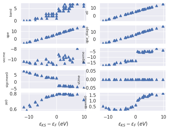
KS Fermi energy at: 5.63275689227251 eV eV
This figure gives us the opportunity to discuss several important points.
First of all the QP correction (qpeme0) are rather smooth so one can try to interpolate the data
with some kind of interpolation algorithm.
Note how valence and conduction states are affected in a different way by the self-energy.
As expected, the matrix elements of the exchange part sigxme
(a.k.a Fock operator in Hartree-Fock theory) are always negative but they also show a “jump” across the Fermi level.
A similar jump is observed in the matrix elements of the correlation part sigcmee0.
These jumps are responsibile for the “opening” of the gap induced by \(GW\).
The values of the renormalization factor ze0 are relatively close to one thus indicating
that we have well-defined QP excitations.
Note how ze0 increases when we approach the Fermi level.
As we are usually interested in the value of the QP direct gaps, let’s plot them with:
sigres.plot_qpgaps();
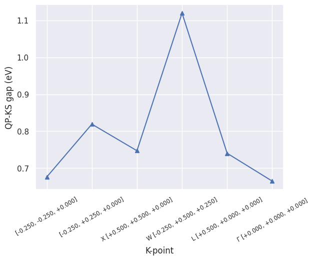
We can also visualize the difference between the QP and the KS values with:
sigres.plot_qpgaps(plot_qpmks=True);

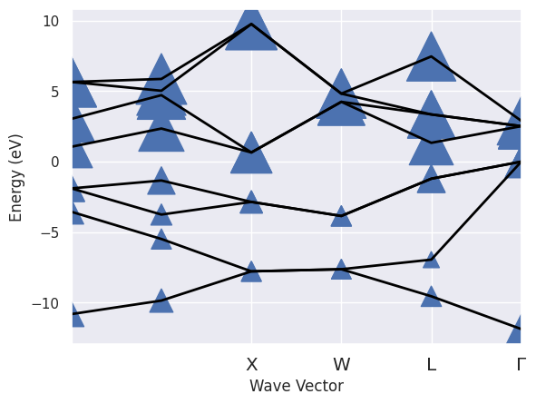
As expected, \(G_0W_0\) leads to a systematic opening of the KS gaps although we should keep in mind that these results are far from being converged.
sigres.plot_ksbands_with_qpmarkers();
Interpolating the QP corrections#
Excellent, we’ve just completed our first \(GW\) calculation with Abinit and Abipy but there’s still a problem that must be addressed!
We can only compute QP energies for k-points belonging to the k-mesh of the input WFK file while we usually discuss electronic properties in terms of band energies along a high-symmetry k-path. Obviously one could perform several different \(GW\) calculations with “shifted” WFK files to collect the QP energies along the k-path but this is not the most efficient approach. Can’t we just use some kind of interpolation technique to get nice-looking QP band structures?
The answer is yes but remember to always cross-check the interpolated results. Several different approaches to interpolate QP results have been proposed in the literature. Here we use the Fourier interpolation scheme proposed by Shankland-Koelling-Wood (SKW) in PRB 38 2721. The idea is relatively simple: the QP corrections have the same symmetry of the KS energies, we can thus interpolate the QP corrections with SKW and then apply the interpolated corrections to the ab-initio KS energies obtained along a path.
It’s just a matter of passing the KS band structure to the sigres.interpolate method to activate this procedure:
r = sigres.interpolate(lpratio=5, ks_ebands_kpath=ks_ebands_kpath)
Using: 30 star-functions. nstars/nk: 5.0
FIT vs input data: Mean Absolute Error= 2.342e-13 (meV)
The interpolated QP band structure is available in r.qp_ebands_kpath and we can plot the interpolated data with:
r.qp_ebands_kpath.plotly();
The results make sense but it would be nice if one could compare the (interpolated) QP bands with the KS energies.
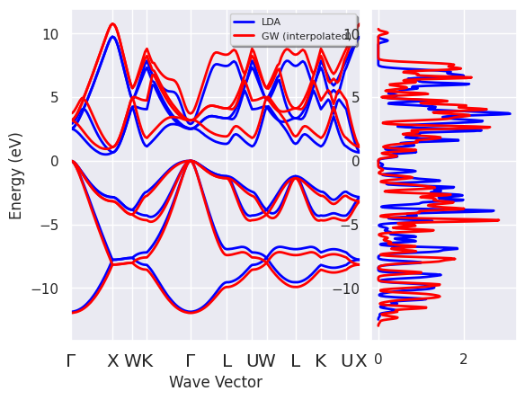
Fortunately, we can use the AbiPy ElectronBandsPlotter to compare multiple band structures:
p = abilab.ElectronBandsPlotter()
p.add_ebands("LDA", ks_ebands_kpath)
p.add_ebands("GW (interpolated)", r.qp_ebands_kpath)
p.combiplot();
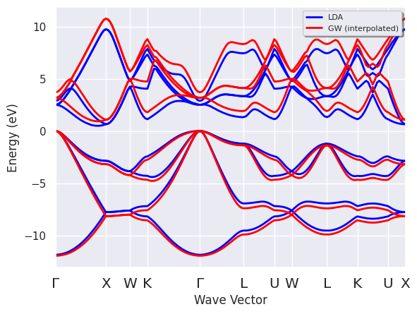
Do you need to compare the band dispersion given by KS and \(GW\)?
# By default, the two band energies are shifted with respect to *their* fermi level.
# Use e=0 if you do not want to shift the eigenvalues
# so that it is possible to visualize the QP corrections.
p.combiboxplot();
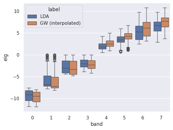
The same approach can be used to interpolate QP band structures and QP DOSes. We only need to pass an additional KS band structure with energies in the IBZ:
r2 = sigres.interpolate(lpratio=5, ks_ebands_kpath=ks_ebands_kpath, ks_ebands_kmesh=ks_ebands_kmesh)
Using: 30 star-functions. nstars/nk: 5.0
FIT vs input data: Mean Absolute Error= 2.342e-13 (meV)
and then compute the QP DOS with:
qp_edos = r2.qp_ebands_kmesh.get_edos()
Did I tell you that ElectronBandsPlotter accepts DOSes as well?
p2 = abilab.ElectronBandsPlotter()
p2.add_ebands("LDA", ks_ebands_kpath, edos=ks_edos)
p2.add_ebands("GW (interpolated)", r.qp_ebands_kpath, edos=qp_edos)
p2.combiplot();
