Base1 lesson (H2 molecule)#
First (basic) lesson with Abinit and AbiPy
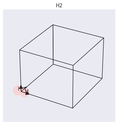
The H2 molecule
This lesson aims at showing how to get the following physical properties:
- the (pseudo) total energy
- the bond length
- the charge density
- the atomisation energy
This tutorial is a complement to the standard ABINIT tutorial on H\(_2\). Here, powerful flow and visualisation procedures will be demonstrated. Still, some basic understanding of the stand-alone working of ABINIT is a prerequisite. Also, in order to fully benefit from this AbiPy tutorial, other more basic AbiPy tutorials should have been followed, as suggested in the introduction page.
There are three methodologies to compute the optimal distance between the two Hydrogen atoms. One could:
compute the total energy for different values of the interatomic distance, make a fit through the different points, and determine the minimum of the fitting function;
compute the forces for different values of the interatomic distance, make a fit through the different values, and determine the zero of the fitting function;
use an automatic algorithm for minimizing the energy (or finding the zero of forces).
In this AbiPy notebook, we will be focusing on the first approach.
More specifically we will build an Flow to compute the energy and the forces in the \(H_2\) molecule
for different values of the interatomic distance.
This exercise will allow us to learn how to generate multiple input files using AbiPy and
how to analyze multiple ground-state calculations with the AbiPy robots.
Note
AbiPy provides two different APIs to produce figures either with matplotlib or with plotly. In this tutorial, we will use the plotly API as much as possible although it should be noted that not all the plotting methods have been yet ported to plotly.
AbiPy uses a relatively simple rule to differentiate between the two plotting libraries:
if an object provides an obj.plot method producing a matplotlib plot, the corresponding
native plotly version (if available) is named obj.plotly.
Note that plotly requires a web browser hence the matplotlib version is still valuable if you need to
visualize results on machines in which only the X-server is available.
In AbiPy versions greater than 0.9, it is possible to try converting matplotlib figures produce by plot methods
into Plotly figures using the optional argument plotly=True, although the result is not always guaranteed.
Warning
In order to run ABINIT executables from AbiPy, you need a manager.yml with configuration options. For further details, please consult the TaskManager documentation.
Our first AbiPy function#
import numpy as np

import warnings
warnings.filterwarnings("ignore")  # Ignore warnings

from abipy import abilab
abilab.enable_notebook() # This line tells AbiPy we are running inside a notebook

# This line configures matplotlib to show figures embedded in the notebook.
# Replace `inline` with `notebook` in classic notebook
%matplotlib inline

# Option available in jupyterlab. See https://github.com/matplotlib/jupyter-matplotlib
#%matplotlib widget
We need a function that generates an input file for a GS calculations for the \(H_2\) molecule in a big box.
Ideally a function that receives the distance x, the cutoff energy ecut and the size of the big box
in input so that we can customize the output and generate multiple input objects easily.
Fortunately we already have such a function in the lesson_base1.py module.
Let’s import it and look at the code:
from lesson_base1 import gs_input
abilab.print_source(gs_input)
def gs_input(x=0.7, ecut=10, acell=(10, 10, 10)):
    """
    This function builds an AbinitInput object to compute the total energy
    of the H2 molecule in a big box.

    Args:
        x: Position of the first Hydrogen along the x-axis in Cartesian coordinates.
           The second Hydrogen is located at [-x, 0, 0]
        ecut: Cutoff energy in Ha.
        acell: Lengths of the primitive vectors (in Bohr)

    Returns:
        AbinitInput object.
    """
    # Build structure from dictionary with input variables.
    structure = abilab.Structure.from_abivars(
        ntypat=1,                           # There is only one type of atom.
        znucl=1,                            # Atomic numbers of the type(s) of atom.
        natom=2,                            # There are two atoms.
        typat=(1, 1),                       # They both are of type 1, that is, Hydrogen.
        xcart=[-x, 0.0, 0.0,                # Cartesian coordinates of atom 1, in Bohr.
               +x, 0.0, 0.0],               # second atom.
        acell=acell,                        # Lengths of the primitive vectors (in Bohr).
        rprim=[1, 0, 0, 0, 1, 0, 0, 0, 1]   # Orthogonal primitive vectors (default).
    )

    # Build AbinitInput from structure and pseudo(s) taken from AbiPy package.
    inp = abilab.AbinitInput(structure=structure, pseudos=abidata.pseudos("01h.pspgth"))

    # Set value of other variables.
    inp.set_vars(
        ecut=ecut,
        nband=1,
        diemac=2.0,
        toldfe=1e-6,
        prtwf=-1,
        iomode=3
    )

    # Define k-point sampling.
    inp.set_kmesh(ngkpt=(1, 1, 1), shiftk=(0, 0, 0))

    return inp
If the function is called without arguments, the default values (specified in the prototype) are used. Let’s try:
gsinp = gs_input()
print("The value of ecut is:", gsinp["ecut"])
The value of ecut is: 10
The AbinitInput is a dict-like object whose usage is documented in this notebook.
Inside jupyter, we can get the HTML representation of the input with:
gsinp
#### SECTION: basic
##############################################
ecut 10
nband 1
toldfe 1e-06
ngkpt 1 1 1
kptopt 1
nshiftk 1
shiftk 0 0 0
##############################################
#### SECTION: dev
##############################################
iomode 3
##############################################
#### SECTION: files
##############################################
prtwf -1
indata_prefix indata/in
tmpdata_prefix tmpdata/tmp
outdata_prefix outdata/out
pseudos /home/runner/work/abipy_book/abipy_book/abipy/abipy/data/pseudos/01h.pspgth
##############################################
#### SECTION: gstate
##############################################
diemac 2.0
##############################################
#### STRUCTURE
##############################################
natom 2
ntypat 1
typat 1 1
znucl 1
xred
-0.0700000000 0.0000000000 0.0000000000
0.0700000000 0.0000000000 0.0000000000
acell 1.0 1.0 1.0
rprim
10.0000000000 0.0000000000 0.0000000000
0.0000000000 10.0000000000 0.0000000000
0.0000000000 0.0000000000 10.0000000000
The input object can be converted into a string.
More importantly, an AbinitInput has an AbiPy structure (see Structure notebook),
a list of pseudopotential objects and provides several methods
to facilitate the specification of input variables.
print(gsinp.structure)
print("The big box volume is:", gsinp.structure.volume)
Full Formula (H2)
Reduced Formula: H2
abc   :   5.291772   5.291772   5.291772
angles:  90.000000  90.000000  90.000000
pbc   :       True       True       True
Sites (2)
  #  SP        a    b    c
---  ----  -----  ---  ---
  0  H     -0.07    0    0
  1  H      0.07    0    0
The big box volume is: 148.1847111705721
gsinp.structure.plot();
Let’s print some info about our pseudopotentials:
print(gsinp.pseudos[0])
<NcAbinitPseudo: 01h.pspgth>
  summary: Goedecker-Teter-Hutter  Wed May  8 14:27:44 EDT 1996
  number of valence electrons: 1.0
  maximum angular momentum: s
  angular momentum for local part: s
  XC correlation: LDA_XC_TETER93
  supports spin-orbit: False
  radius for non-linear core correction: 0.0
  hint for low accuracy: ecut: 0.0, pawecutdg: 0.0
  hint for normal accuracy: ecut: 0.0, pawecutdg: 0.0
  hint for high accuracy: ecut: 0.0, pawecutdg: 0.0
Computation of the interatomic distance#
At this point, we can use gs_input to generate an Abinit Flow
to compute the total energy and the forces of H-H with different interatomic distances.
We have already prepared such a function in build_flow, let’s have a look at the code:
from lesson_base1 import build_flow
abilab.print_source(build_flow)
def build_flow(options):
    """
    Generate a flow to compute the total energy and forces for the H2 molecule in a big box
    as a function of the interatomic distance.

    Args:
        options: Command line options.

    Return:
        Flow object.
    """
    inputs = [gs_input(x=x) for x in np.linspace(0.5, 1.025, 21)]

    workdir = options.workdir if (options and options.workdir) else "flow_h2"

    return flowtk.Flow.from_inputs(workdir, inputs)
Note that we are working at fixed ecut and acell, only the H-H distance is modified. Let’s call the function to build our flow:
flow = build_flow(options=None)
flow.get_graphviz()

Ok, so far so good.
With just three lines of codes and our gs_input function, we managed
to construct an AbiPy flow for the \(H_2\) molecule.
Let’s write some python code to check that we really obtained what we had in mind:
inputs = [task.input for task in flow.iflat_tasks()]

print("ecuts:\n", [inp["ecut"] for inp in inputs])

print("vols:\n", ["%.1f" % inp.structure.volume for inp in inputs])

def hh_dist(structure):
    return np.linalg.norm(structure.cart_coords[1] - structure.cart_coords[0])

from pprint import pprint
print("h-h [Ang]:\n", ["%.3f" % hh_dist(inp.structure) for inp in inputs])
ecuts:
 [10, 10, 10, 10, 10, 10, 10, 10, 10, 10, 10, 10, 10, 10, 10, 10, 10, 10, 10, 10, 10]
vols:
 ['148.2', '148.2', '148.2', '148.2', '148.2', '148.2', '148.2', '148.2', '148.2', '148.2', '148.2', '148.2', '148.2', '148.2', '148.2', '148.2', '148.2', '148.2', '148.2', '148.2', '148.2']
h-h [Ang]:
 ['0.529', '0.557', '0.585', '0.613', '0.640', '0.668', '0.696', '0.724', '0.751', '0.779', '0.807', '0.835', '0.863', '0.890', '0.918', '0.946', '0.974', '1.001', '1.029', '1.057', '1.085']
At this point, we could run the flow in the notebook by just calling:
flow.make_scheduler().start()
or, alternatively, execute the lesson_base1.py script to build
the directory with the flow and then use:
abirun.py flow_h2 scheduler
inside the terminal.
Let’s assume the flow has been already executed and let’s focus on the analysis of the final results.
Analyzing the main output file#
First of all, it is always a good idea to check whether the SCF cycle is converged. Obviously one could open the main output file, find the SCF iterations and look for warnings but there is a much faster (and better) way to do that with AbiPy:
abo = abilab.abiopen("flow_h2/w0/t0/run.abo")
print(abo)
ndtset: 1, completed: True
Full Formula (H2)
Reduced Formula: H2
abc   :   5.291772   5.291772   5.291772
angles:  90.000000  90.000000  90.000000
pbc   :       True       True       True
Sites (2)
  #  SP        a    b    c
---  ----  -----  ---  ---
  0  H     -0.05    0    0
  1  H      0.05    0    0

Abinit Spacegroup: spgid: 123, num_spatial_symmetries: 16, has_timerev: True, symmorphic: False

========================= Dimensions of calculation =========================
         intxc  ionmov  iscf  lmnmax  lnmax  mgfft  mpssoang  mqgrid  natom  \
dataset
1            0       0     7       1      1     30         1    3001      2

         nloc_mem  nspden  nspinor  nsppol  nsym  n1xccc  ntypat  occopt  \
dataset
1               1       1        1       1    16       0       1       1

         xclevel  mband  mffmem  mkmem  mpw   nfft  nkpt  mem_per_proc_mb  \
dataset
1              1      1       1      1  752  27000     1            7.796

         wfk_size_mb  denpot_size_mb spg_symbol  spg_number  \
dataset
1              0.013           0.208     P4/mmm         123

                                bravais
dataset
1        Bravais tP (primitive tetrag.)
To get the list of Warnings/Comments/Errors:
print(abo.events)
Events found in /home/runner/work/abipy_book/abipy_book/abipy_book/base1/flow_h2/w0/t0/run.abo

num_errors: 0, num_warnings: 0, num_comments: 0, completed: False
To plot the SCF cycle, use:
abo.plot();
Loading all matplotlib figures before showing them. It may take some time...
All figures in memory, elapsed time: 0.251 s

Since this is not a structural relaxation, the initial and final structures must be equal:
abo.initial_structure == abo.final_structure
True
The basic dimensions and parameters of the run can be extracted from the output file with:
abo.get_dims_spginfo_dataset()
({1: {'intxc': 0,
   'ionmov': 0,
   'iscf': 7,
   'lmnmax': 1,
   'lnmax': 1,
   'mgfft': 30,
   'mpssoang': 1,
   'mqgrid': 3001,
   'natom': 2,
   'nloc_mem': 1,
   'nspden': 1,
   'nspinor': 1,
   'nsppol': 1,
   'nsym': 16,
   'n1xccc': 0,
   'ntypat': 1,
   'occopt': 1,
   'xclevel': 1,
   'mband': 1,
   'mffmem': 1,
   'mkmem': 1,
   'mpw': 752,
   'nfft': 27000,
   'nkpt': 1,
   'mem_per_proc_mb': 7.796,
   'wfk_size_mb': 0.013,
   'denpot_size_mb': 0.208}},
 {1: {'spg_symbol': 'P4/mmm',
   'spg_number': 123,
   'bravais': 'Bravais tP (primitive tetrag.)'}})
Within the shell, one can use:
abiview.py abo flow_h2/w0/t0/run.abo
to plot the SCF cycle or
abiopen.py flow_h2/w0/t0/run.abo
to open the file and start the ipython terminal
Note that the object returned by abiopen has an associated file descriptor that should be closed
explicitly by the user with abo.close().
This is the reason why many examples will use the python context manager:
    with abiopen("path") as abifile:
        print(abifile)
that closes the file when we exit the with block.
Extracting results from the GSR files#
The ground-state results are saved in the GSR.nc files whose API is extensively
discussed in the GSR notebook.
Let’s have a look at the results produced by the first task:
with abilab.abiopen("flow_h2/w0/t0/outdata/out_GSR.nc") as gsr:
    print(gsr)
================================= File Info =================================
Name: out_GSR.nc
Directory: /home/runner/work/abipy_book/abipy_book/abipy_book/base1/flow_h2/w0/t0/outdata
Size: 8.20 kB
Access Time: Thu Jan 15 12:16:16 2026
Modification Time: Thu Jan 15 12:13:03 2026
Change Time: Thu Jan 15 12:13:03 2026

================================= Structure =================================
Full Formula (H2)
Reduced Formula: H2
abc   :   5.291772   5.291772   5.291772
angles:  90.000000  90.000000  90.000000
pbc   :       True       True       True
Sites (2)
  #  SP        a    b    c  cartesian_forces
---  ----  -----  ---  ---  --------------------------------------------------
  0  H     -0.05    0    0  [-19.54779682  -0.          -0.        ] eV ang^-1
  1  H      0.05    0    0  [19.54779682 -0.         -0.        ] eV ang^-1
min |F_iat|: 19.547796823042827 eV/Ang
max |F_iat|: 19.547796823042827 eV/Ang
mean F_iat|: 19.547796823042827 eV/Ang
std  |F_iat|: 0.0 eV/Ang
FORCES ARE NOT FULLY RELAXED. THIS STRUCTURE SHOULD NOT BE USED FOR PHONONS!

Abinit Spacegroup: spgid: 123, num_spatial_symmetries: 16, has_timerev: True, symmorphic: False

Stress tensor (Cartesian coordinates in GPa):
[[-10.75762969   0.           0.        ]
 [  0.           1.60903288   0.        ]
 [  0.           0.           1.60903288]]

Pressure: 2.513 (GPa)
Energy: -28.21337450 (eV)

============================== Electronic Bands ==============================
Number of electrons: 2.0, Fermi level: -11.082 (eV)
nsppol: 1, nkpt: 1, mband: 1, nspinor: 1, nspden: 1
smearing scheme: none (occopt 1), tsmear_eV: 0.272, tsmear Kelvin: 3157.7
Bandwidth: 0.000 (eV)
Valence maximum located at kpt index 0:
    spin: 0, kpt: $\Gamma$ [+0.000, +0.000, +0.000], band: 0, eig: -11.082, occ: 2.000
TIP: Use `--verbose` to print k-point coordinates with more digits
As we can see from the previous output, the GSR file contains information about
the crystalline structure, forces, stresses as well as the KS band structure.
In the jargon of object-oriented programming, one says that a GsrFile has a Structure object:
gsr.structure
and has an ElectronBands object:
gsr.ebands
This means that if you learn how to use the methods provided by structure and ebands, then you can
easily get these objects from the GSR file and use this API to post-process the results.
This is a general philosophy of AbiPy: every netcdf file object returned by abiopen contains
other objects (the structure is always available, while the presence of other objects depend of the particular file).
Remember this important point because we will use it a lot in the other lessons.
Note
To learn about the different methods provided by structure and ebands, you may want to
consult the API documentation
Ok, now we know how to open and extract information from one GSR file.
In this tutorial, however, we need to analyze multiple GSR files!
If you are familiar with python, it should not be difficult to write a for loop that
iterates over a list of GSR files, extracts the total energy with the corresponding volume and creates two
lists that can be used to plot \(E(d)\) with d the H-H distance.
This kind of operations are, however, very common and AbiPy provides a high-level interface (robots) to
operate on multiple files and post-process the data.
In the simplest case, one can use the from_dir method to tell the Robot to
find all files of a particular type located within a directory tree,
and store all the data in memory:
robot = abilab.GsrRobot.from_dir("flow_h2")
robot
- w0/t19/outdata/out_GSR.nc
- w0/t13/outdata/out_GSR.nc
- w0/t12/outdata/out_GSR.nc
- w0/t6/outdata/out_GSR.nc
- w0/t1/outdata/out_GSR.nc
- w0/t10/outdata/out_GSR.nc
- w0/t5/outdata/out_GSR.nc
- w0/t18/outdata/out_GSR.nc
- w0/t11/outdata/out_GSR.nc
- w0/t0/outdata/out_GSR.nc
- w0/t16/outdata/out_GSR.nc
- w0/t9/outdata/out_GSR.nc
- w0/t15/outdata/out_GSR.nc
- w0/t20/outdata/out_GSR.nc
- w0/t4/outdata/out_GSR.nc
- w0/t17/outdata/out_GSR.nc
- w0/t14/outdata/out_GSR.nc
- w0/t2/outdata/out_GSR.nc
- w0/t3/outdata/out_GSR.nc
- w0/t8/outdata/out_GSR.nc
- w0/t7/outdata/out_GSR.nc
Once we have constructed the robot, we can start to invoke methods to extract/post-process the results. For instance, we can construct a pandas Dataframe with:
table = robot.get_dataframe()
The table contains several columns:
table.keys()
Index(['formula', 'natom', 'alpha', 'beta', 'gamma', 'a', 'b', 'c', 'volume',
       'abispg_num', 'spglib_symb', 'spglib_num', 'spglib_lattice_type',
       'energy', 'energy_per_atom', 'pressure', 'max_force', 'ecut',
       'pawecutdg', 'tsmear', 'nkpt', 'nsppol', 'nspinor', 'nspden'],
      dtype='object')
Inside the notebook, we can visualize the table with:
table
| formula | natom | alpha | beta | gamma | a | b | c | volume | abispg_num | ... | energy_per_atom | pressure | max_force | ecut | pawecutdg | tsmear | nkpt | nsppol | nspinor | nspden | |
|---|---|---|---|---|---|---|---|---|---|---|---|---|---|---|---|---|---|---|---|---|---|
| w0/t19/outdata/out_GSR.nc | H2 | 2 | 90.0 | 90.0 | 90.0 | 5.291772 | 5.291772 | 5.291772 | 148.184711 | 123 | ... | -14.788854 | -2.367714 | 3.356837 | 10.0 | -1.0 | 0.01 | 1 | 1 | 1 | 1 |
| w0/t13/outdata/out_GSR.nc | H2 | 2 | 90.0 | 90.0 | 90.0 | 5.291772 | 5.291772 | 5.291772 | 148.184711 | 123 | ... | -15.007564 | -1.650521 | 1.652942 | 10.0 | -1.0 | 0.01 | 1 | 1 | 1 | 1 |
| w0/t12/outdata/out_GSR.nc | H2 | 2 | 90.0 | 90.0 | 90.0 | 5.291772 | 5.291772 | 5.291772 | 148.184711 | 123 | ... | -15.027449 | -1.486643 | 1.198657 | 10.0 | -1.0 | 0.01 | 1 | 1 | 1 | 1 |
| w0/t6/outdata/out_GSR.nc | H2 | 2 | 90.0 | 90.0 | 90.0 | 5.291772 | 5.291772 | 5.291772 | 148.184711 | 123 | ... | -14.953205 | -0.079134 | 3.837290 | 10.0 | -1.0 | 0.01 | 1 | 1 | 1 | 1 |
| w0/t1/outdata/out_GSR.nc | H2 | 2 | 90.0 | 90.0 | 90.0 | 5.291772 | 5.291772 | 5.291772 | 148.184711 | 123 | ... | -14.348841 | 1.960239 | 15.457585 | 10.0 | -1.0 | 0.01 | 1 | 1 | 1 | 1 |
| w0/t10/outdata/out_GSR.nc | H2 | 2 | 90.0 | 90.0 | 90.0 | 5.291772 | 5.291772 | 5.291772 | 148.184711 | 123 | ... | -15.045641 | -1.106892 | 0.050198 | 10.0 | -1.0 | 0.01 | 1 | 1 | 1 | 1 |
| w0/t5/outdata/out_GSR.nc | H2 | 2 | 90.0 | 90.0 | 90.0 | 5.291772 | 5.291772 | 5.291772 | 148.184711 | 123 | ... | -14.889757 | 0.249295 | 5.346041 | 10.0 | -1.0 | 0.01 | 1 | 1 | 1 | 1 |
| w0/t18/outdata/out_GSR.nc | H2 | 2 | 90.0 | 90.0 | 90.0 | 5.291772 | 5.291772 | 5.291772 | 148.184711 | 123 | ... | -14.834181 | -2.273618 | 3.164346 | 10.0 | -1.0 | 0.01 | 1 | 1 | 1 | 1 |
| w0/t11/outdata/out_GSR.nc | H2 | 2 | 90.0 | 90.0 | 90.0 | 5.291772 | 5.291772 | 5.291772 | 148.184711 | 123 | ... | -15.040523 | -1.306064 | 0.669857 | 10.0 | -1.0 | 0.01 | 1 | 1 | 1 | 1 |
| w0/t0/outdata/out_GSR.nc | H2 | 2 | 90.0 | 90.0 | 90.0 | 5.291772 | 5.291772 | 5.291772 | 148.184711 | 123 | ... | -14.106687 | 2.513188 | 19.547797 | 10.0 | -1.0 | 0.01 | 1 | 1 | 1 | 1 |
| w0/t16/outdata/out_GSR.nc | H2 | 2 | 90.0 | 90.0 | 90.0 | 5.291772 | 5.291772 | 5.291772 | 148.184711 | 123 | ... | -14.915720 | -2.058169 | 2.682742 | 10.0 | -1.0 | 0.01 | 1 | 1 | 1 | 1 |
| w0/t9/outdata/out_GSR.nc | H2 | 2 | 90.0 | 90.0 | 90.0 | 5.291772 | 5.291772 | 5.291772 | 148.184711 | 123 | ... | -15.041404 | -0.887078 | 0.681054 | 10.0 | -1.0 | 0.01 | 1 | 1 | 1 | 1 |
| w0/t15/outdata/out_GSR.nc | H2 | 2 | 90.0 | 90.0 | 90.0 | 5.291772 | 5.291772 | 5.291772 | 148.184711 | 123 | ... | -14.950974 | -1.934773 | 2.386232 | 10.0 | -1.0 | 0.01 | 1 | 1 | 1 | 1 |
| w0/t20/outdata/out_GSR.nc | H2 | 2 | 90.0 | 90.0 | 90.0 | 5.291772 | 5.291772 | 5.291772 | 148.184711 | 123 | ... | -14.741056 | -2.453928 | 3.520449 | 10.0 | -1.0 | 0.01 | 1 | 1 | 1 | 1 |
| w0/t4/outdata/out_GSR.nc | H2 | 2 | 90.0 | 90.0 | 90.0 | 5.291772 | 5.291772 | 5.291772 | 148.184711 | 123 | ... | -14.803196 | 0.612993 | 7.176415 | 10.0 | -1.0 | 0.01 | 1 | 1 | 1 | 1 |
| w0/t17/outdata/out_GSR.nc | H2 | 2 | 90.0 | 90.0 | 90.0 | 5.291772 | 5.291772 | 5.291772 | 148.184711 | 123 | ... | -14.876621 | -2.170734 | 2.940714 | 10.0 | -1.0 | 0.01 | 1 | 1 | 1 | 1 |
| w0/t14/outdata/out_GSR.nc | H2 | 2 | 90.0 | 90.0 | 90.0 | 5.291772 | 5.291772 | 5.291772 | 148.184711 | 123 | ... | -14.981811 | -1.799429 | 2.045489 | 10.0 | -1.0 | 0.01 | 1 | 1 | 1 | 1 |
| w0/t2/outdata/out_GSR.nc | H2 | 2 | 90.0 | 90.0 | 90.0 | 5.291772 | 5.291772 | 5.291772 | 148.184711 | 123 | ... | -14.539636 | 1.463278 | 12.125932 | 10.0 | -1.0 | 0.01 | 1 | 1 | 1 | 1 |
| w0/t3/outdata/out_GSR.nc | H2 | 2 | 90.0 | 90.0 | 90.0 | 5.291772 | 5.291772 | 5.291772 | 148.184711 | 123 | ... | -14.688544 | 1.016114 | 9.404751 | 10.0 | -1.0 | 0.01 | 1 | 1 | 1 | 1 |
| w0/t8/outdata/out_GSR.nc | H2 | 2 | 90.0 | 90.0 | 90.0 | 5.291772 | 5.291772 | 5.291772 | 148.184711 | 123 | ... | -15.026087 | -0.644270 | 1.549818 | 10.0 | -1.0 | 0.01 | 1 | 1 | 1 | 1 |
| w0/t7/outdata/out_GSR.nc | H2 | 2 | 90.0 | 90.0 | 90.0 | 5.291772 | 5.291772 | 5.291772 | 148.184711 | 123 | ... | -14.997564 | -0.375908 | 2.588480 | 10.0 | -1.0 | 0.01 | 1 | 1 | 1 | 1 |
21 rows × 24 columns
Great! We managed to get a nice table with lot of useful results with just three lines of code and the robot! There are however two problems:
The rows of the table are not ordered by increasing H-H distance (files are sorted alphabetically)
Our dataframe contains the energy of the different configurations, but we would like to plot the energy as a function of the H-H distance
Well, robots can do a lot of hard work but they are a little bit stupid so
we have to tell them what to do with the data.
More specifically we need a way to tell the robot that, for each GSR file, it should get the crystalline
structure, compute the distance between the first and the second atom and insert the result
in our table in a given column.
This kind of tasks are usually executed with callbacks i.e. functions that are passed in input
and automatically executed by the framework at runtime.

Let’s look at the documentation of robot.get_dataframe:
abilab.print_doc(robot.get_dataframe)
    def get_dataframe(self, with_geo=True, abspath=False, with_paths=True, funcs=None, **kwargs) -> pd.DataFrame:
        """
        Return a |pandas-DataFrame| with the most important GS results and the filenames as index.

        Args:
            with_geo: True if structure info should be added to the dataframe
            abspath: True if paths in the index should be absolute. Default: Relative to getcwd().
            with_paths: False if filepaths should not be added

        kwargs:
            attrs:
                List of additional attributes of the |GsrFile| to add to the DataFrame.
            funcs: Function or list of functions to execute to add more data to the DataFrame.
                Each function receives a |GsrFile| object and returns a tuple (key, value)
                where key is a string with the name of column and value is the value to be inserted.
        """
It seems complicated but the actual implementation of the callback is just three lines of code:
def hh_dist(gsr):
    """
    This callback receives a GSR file and computes the H-H distance.
    The robot will call this function to compute the H-H distance,
    and return a (key, value) tuple that will be inserted in the pandas DataFrame.
    """
    cart_coords = gsr.structure.cart_coords
    d = np.linalg.norm(cart_coords[1] - cart_coords[0])
    return "hh_dist", d

with abilab.GsrRobot.from_dir("flow_h2") as robot:
    table = robot.get_dataframe(funcs=hh_dist)
    table = table.sort_values(by="hh_dist")
As expected, now the table contains a new column with hh_dist in Angstrom:
"hh_dist" in table
True
Let’s print the two columns with the H-H distance and the total energy:
table[["hh_dist", "energy"]]
| hh_dist | energy | |
|---|---|---|
| w0/t0/outdata/out_GSR.nc | 0.529177 | -28.213374 |
| w0/t1/outdata/out_GSR.nc | 0.556959 | -28.697681 |
| w0/t2/outdata/out_GSR.nc | 0.584741 | -29.079272 |
| w0/t3/outdata/out_GSR.nc | 0.612523 | -29.377087 |
| w0/t4/outdata/out_GSR.nc | 0.640304 | -29.606393 |
| w0/t5/outdata/out_GSR.nc | 0.668086 | -29.779514 |
| w0/t6/outdata/out_GSR.nc | 0.695868 | -29.906409 |
| w0/t7/outdata/out_GSR.nc | 0.723650 | -29.995127 |
| w0/t8/outdata/out_GSR.nc | 0.751432 | -30.052174 |
| w0/t9/outdata/out_GSR.nc | 0.779213 | -30.082807 |
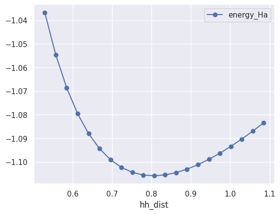
| w0/t10/outdata/out_GSR.nc | 0.806995 | -30.091282 |
| w0/t11/outdata/out_GSR.nc | 0.834777 | -30.081045 |
| w0/t12/outdata/out_GSR.nc | 0.862559 | -30.054898 |
| w0/t13/outdata/out_GSR.nc | 0.890341 | -30.015128 |
| w0/t14/outdata/out_GSR.nc | 0.918122 | -29.963621 |
| w0/t15/outdata/out_GSR.nc | 0.945904 | -29.901949 |
| w0/t16/outdata/out_GSR.nc | 0.973686 | -29.831440 |
| w0/t17/outdata/out_GSR.nc | 1.001468 | -29.753241 |
| w0/t18/outdata/out_GSR.nc | 1.029250 | -29.668361 |
| w0/t19/outdata/out_GSR.nc | 1.057031 | -29.577707 |
| w0/t20/outdata/out_GSR.nc | 1.084813 | -29.482112 |
Note that the energy in our DataFrame is given in eV to facilitate the integration
with pymatgen that uses eV for energies and Angstrom for lengths.
Let’s add another column to our table with energies in Hartree:
table["energy_Ha"] = table["energy"] * abilab.units.eV_to_Ha
and use the plot method of pandas DataFrames to plot energy_Ha vs hh_dist
table.plot(x="hh_dist", y="energy_Ha", style="-o");
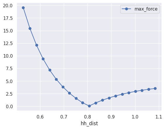
At this point, it should be clear that to plot the maximum of the forces as a function of the H-H distance we just need:
table.plot(x="hh_dist", y="max_force", style="-o");
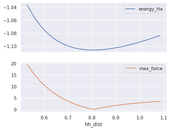
Want to plot the two quantities on the same figure?
table.plot(x="hh_dist", y=["energy_Ha", "max_force"], subplots=True);
Note
Your boss understands the data only if it is formatted inside a \(\LaTeX\) tabular environment?
table[["hh_dist", "energy"]].to_latex()
Need to send data to Windows users?
table.to_excel("'output.xlsx")
Want to copy the dataframe to the system clipboard so that one can easily past the data into an other applications e.g. Excel?
table.to_clipboard()
Analysis of the charge density#
The DEN.nc file stores the density in real space on the FFT mesh.
A DEN.nc file has a structure, and an ebands object with the electronic eigenvalues/occupations
and a Density object with \(n(r)\) (numpy array .datar) and \(n(G)\) (.datag).
Let’s open the file with abiopen and print it:
with abilab.abiopen("flow_h2/w0/t10/outdata/out_DEN.nc") as denfile:
    print(denfile)
    density = denfile.density
================================= File Info =================================
Name: out_DEN.nc
Directory: /home/runner/work/abipy_book/abipy_book/abipy_book/base1/flow_h2/w0/t10/outdata
Size: 217.43 kB
Access Time: Thu Jan 15 12:16:17 2026
Modification Time: Thu Jan 15 12:13:03 2026
Change Time: Thu Jan 15 12:13:03 2026

================================= Structure =================================
Full Formula (H2)
Reduced Formula: H2
abc   :   5.291772   5.291772   5.291772
angles:  90.000000  90.000000  90.000000
pbc   :       True       True       True
Sites (2)
  #  SP           a    b    c
---  ----  --------  ---  ---
  0  H     -0.07625    0    0
  1  H      0.07625    0    0

Abinit Spacegroup: spgid: 123, num_spatial_symmetries: 16, has_timerev: True, symmorphic: False

============================== Electronic Bands ==============================
Number of electrons: 2.0, Fermi level: -9.658 (eV)
nsppol: 1, nkpt: 1, mband: 1, nspinor: 1, nspden: 1
smearing scheme: none (occopt 1), tsmear_eV: 0.272, tsmear Kelvin: 3157.7
Bandwidth: 0.000 (eV)
Valence maximum located at kpt index 0:
    spin: 0, kpt: $\Gamma$ [+0.000, +0.000, +0.000], band: 0, eig: -9.658, occ: 2.000
TIP: Use `--verbose` to print k-point coordinates with more digits
XC functional: LDA_XC_TETER93
================================== Density ==================================
Density: nspinor: 1, nsppol: 1, nspden: 1
Mesh3D: nx=30, ny=30, nz=30
Integrated electronic and magnetization densities in atomic spheres:
      symbol      ntot  rsph_ang           frac_coords
iatom
0          H  0.134448      0.31  [-0.07625, 0.0, 0.0]
1          H  0.134448      0.31   [0.07625, 0.0, 0.0]
Total magnetization from unit cell integration: 0.0
The simplest thing we can do now is to print \(n(r)\) along a line passing through two points specified
either in terms of two vectors or two integers defining the site index in our structure.
Let’s plot the density along the H-H bond by passing the index of the two atoms:
density.plot_line(0, 1);

Great! If we have a netcdf file and AbiPy, we don’t need to use cut3d to extract the data from the file
and we can do simple plots with matplotlib.
Unfortunately, \(n(r)\) is a 3D object and the notebook is not the most suitable tool to visualize this kind of dataset.
Fortunately there are several graphical applications to visualize 3D fields in crystalline environments
and AbiPy provides tools to export the data from netcdf to the text format supported by the external graphical tool.
For example, one can use:
#density.visualize("vesta")
to visualize density isosurfaces of our system:

Conclusions#
To summarize, we learned how to define python functions that can be used to generate many input files easily.
We briefly discussed how to use these inputs to build a basic AbiPy flow without dependencies.
More importantly, we showed that AbiPy provides several tools that can be used to inspect and analyze
the results without having to pass necessarily through the creation and execution of the Flow.
Last but not least, we discussed how to use robots to collect results from the output files and store
them in pandas DataFrames.
AbiPy users are strongly recommended to familiarize themself with this kind of interface before moving to more advanced features such as the flow execution that requires a good understanding of the python language. As a matter of fact, we decided to write AbiPy in python not for efficiency reasons (actually python is usually slower that Fortran/C) but because there are tons of libraries for scientific applications (numpy, scipy, pandas, matplotlib, jupyter, etc). If you learn to use these great libraries for your work you can really boost your productivity and save a lot of time.
A logical next lesson would be the the tutorial about the ground-state properties of silicon