Potentials

This example shows how to plot the potentials stored in netcdf files. Use the input variables prtpot, prtvha, prtvhxc, prtvxc with iomode 3 to produce these files at the end of the SCF-GS run.

• 
• 
• 
• 

from abipy.abilab import abiopen
import abipy.data as abidata

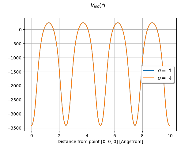
# VKS = Hartree + XC potential + sum of local part of pseudos.
with abiopen(abidata.ref_file("ni_666k_POT.nc")) as ncfile:
    vks = ncfile.vks

#vks.plot_line(point1=[0, 0, 0], point2=[0, 4, 0], num=400, title="$V_{ks}(r)$")

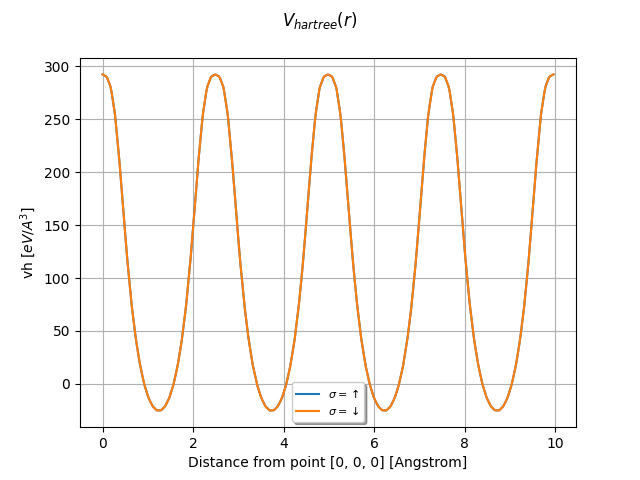
# Hartree potential.
with abiopen(abidata.ref_file("ni_666k_VHA.nc")) as ncfile:
    vh = ncfile.vh

vh.plot_line(point1=[0, 0, 0], point2=[0, 4, 0], num=400, title="$V_{hartree}(r)$")

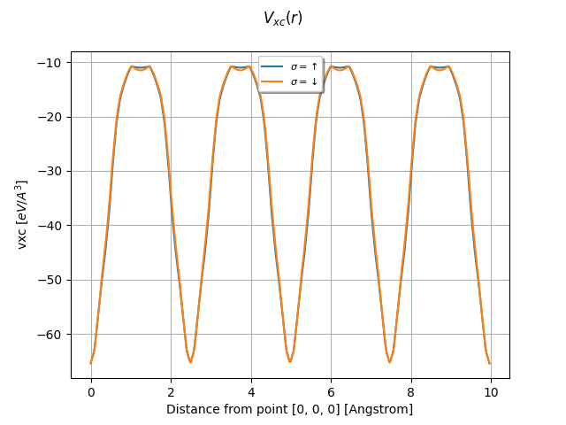
# XC potential.
with abiopen(abidata.ref_file("ni_666k_VXC.nc")) as ncfile:
    vxc = ncfile.vxc

vxc.plot_line(point1=[0, 0, 0], point2=[0, 4, 0], num=400, title="$V_{xc}(r)$")

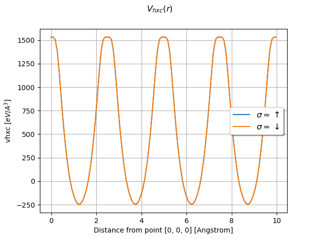
# Hartree + XC potential.
with abiopen(abidata.ref_file("ni_666k_VHXC.nc")) as ncfile:
    vhxc = ncfile.vhxc

vhxc.plot_line(point1=[0, 0, 0], point2=[0, 4, 0], num=400, title="$V_{hxc}(r)$")

vloc = vks - vhxc
vloc.plot_line(point1=[0, 0, 0], point2=[0, 4, 0], num=400, title="$V_{loc}(r)$")

foo = vhxc - vh - vxc
#foo.plot_line(point1=[0, 0, 0], point2=[0, 4, 0], num=400, title="$V_{hxc - h - xc}(r)$")

# To plot the wavefunction along the lines connect the firt atom in the structure
# and all the neighbors within a sphere of radius 3 Angstrom:
#vxc.plot_line_neighbors(site_index=0, radius=3)