GW corrections

This example shows how to interpolate the GW corrections and use the interpolated values to correct the KS band structure computed on a high symmetry k-path and the KS energies of a k-mesh. Finally, the KS and the GW results are plotted with matplotlib.

• 
• 
• 
• 
• 

Using: 30 star-functions. nstars/nk: 5.0
FIT vs input data: Mean Absolute Error= 1.523e-13 (meV)

import abipy.data as abidata
from abipy.abilab import abiopen, ElectronBandsPlotter

# Get quasiparticle results from the SIGRES.nc database.
sigres = abiopen(abidata.ref_file("si_g0w0ppm_nband30_SIGRES.nc"))

# Read the KS band energies computed on the k-path
with abiopen(abidata.ref_file("si_nscf_GSR.nc")) as gsr_nscf:
    ks_ebands_kpath = gsr_nscf.ebands

# Read the KS band energies computed on the Monkhorst-Pack (MP) mesh
# and compute the DOS with the Gaussian method
with abiopen(abidata.ref_file("si_scf_GSR.nc")) as gsr_scf:
    ks_ebands_kmesh = gsr_scf.ebands

ks_edos = ks_ebands_kmesh.get_edos()

# Interpolate the QP corrections and use the interpolated values to correct
# the KS energies stored in `ks_ebands_kpath` and `ks_ebands_kmesh`.
#
# The QP energies are returned in r.qp_ebands_kpath and r.qp_ebands_kmesh.
# Note that the KS energies are optional but this is the recommended approach
# because the code will interpolate the corrections instead of the QP energies.

r = sigres.interpolate(lpratio=5,
                       ks_ebands_kpath=ks_ebands_kpath,
                       ks_ebands_kmesh=ks_ebands_kmesh
                       )
qp_edos = r.qp_ebands_kmesh.get_edos()

# Get points with ab-initio QP energies from the SIGRES so that
# we can plot the interpolate interpolated QP band structure with the first principles results.
# This part is optional
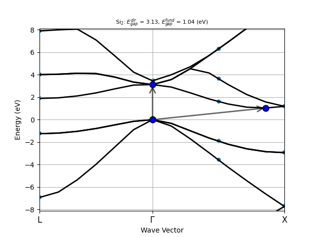
points = sigres.get_points_from_ebands(r.qp_ebands_kpath, size=24)
r.qp_ebands_kpath.plot(points=points, with_gaps=True)
#raise ValueError()

# Shortcut: pass the name of the GSR files directly.
#r = sigres.interpolate(ks_ebands_kpath=abidata.ref_file("si_nscf_GSR.nc"),
#                       ks_ebands_kmesh=abidata.ref_file("si_scf_GSR.nc"))
#ks_edos = r.ks_ebands_kmesh.get_edos()
#qp_edos = r.qp_ebands_kmesh.get_edos()

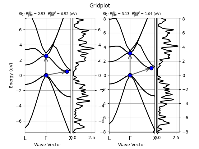
# Use ElectronBandsPlotter to plot the KS and the QP band structure with matplotlib.
plotter = ElectronBandsPlotter()
plotter.add_ebands("LDA", ks_ebands_kpath, edos=ks_edos)
plotter.add_ebands("GW (interpolated)", r.qp_ebands_kpath, edos=qp_edos)

# Get pandas dataframe with band structure parameters.
#df = plotter.get_ebands_frame()
#print(df)

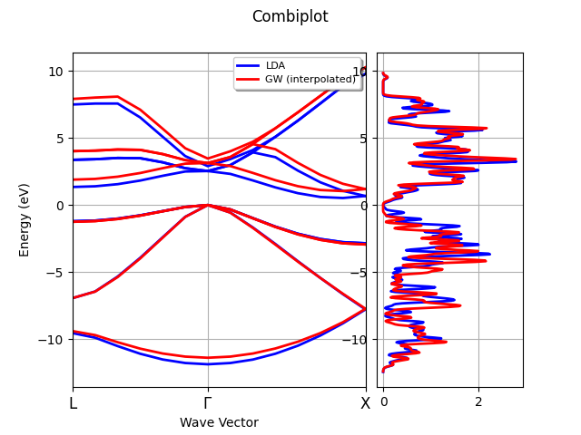
# By default, the two band energies are shifted wrt to *their* fermi level.
# Use e=0 if you don't want to shift the eigenvalus
# so that it's possible to visualize the QP corrections.
plotter.combiplot(title="Combiplot")
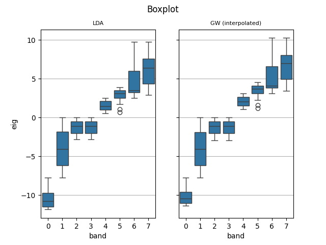
plotter.boxplot(swarm=True, title="Boxplot")
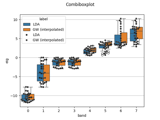
plotter.combiboxplot(swarm=True, title="Combiboxplot")
# sphinx_gallery_thumbnail_number = 4
plotter.gridplot(title="Gridplot", with_gaps=True)

sigres.close()