Bethe-Salpeter

This example shows how to plot the macroscopic dielectric function (MDF) computed in the Bethe-Salpeter code.

• 
• 
• 
• 

import abipy.data as abidata
from abipy.abilab import abiopen

# Open the MDF file produced in the tutorial.
mdf_file = abiopen(abidata.ref_file("tbs_4o_DS2_MDF.nc"))

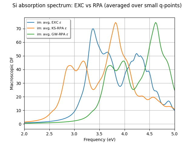
# Plot the imaginary part of the macroscopic
# dielectric function (EXC, RPA, GWRPA) between 2 and 5 eV.
xlims = (2, 5)

mdf_file.plot_mdfs(xlims=xlims,
                   title="Si absorption spectrum: EXC vs RPA (averaged over small q-points)")

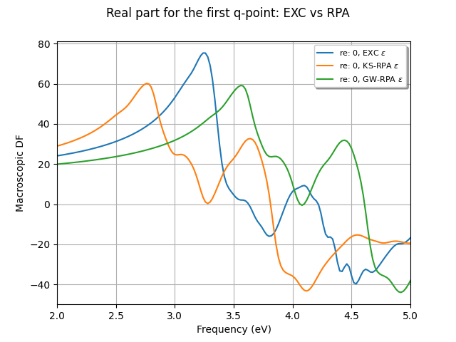
# Plot the real part for the first q-point --> 0
mdf_file.plot_mdfs(cplx_mode="Re", qpoint=0, xlims=xlims,
                   title="Real part for the first q-point: EXC vs RPA")

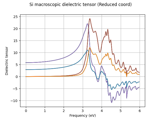
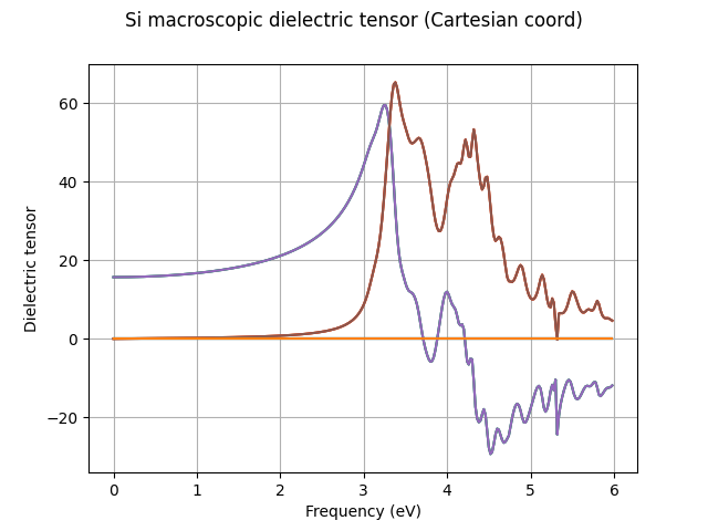
# Plot the 6 different components of the macroscopic dielectric tensor
tensor_exc = mdf_file.get_tensor("exc")
tensor_exc.symmetrize(mdf_file.structure)
tensor_exc.plot(title="Si macroscopic dielectric tensor (Reduced coord)")

tensor_exc.plot(red_coords=False,
                title="Si macroscopic dielectric tensor (Cartesian coord)")

mdf_file.close()