Gruneisen parameters

This example shows how to analyze the Gruneisen parameters computed by anaddb via finite difference. See also v8/Input/t45.in

• 
• 
• 
• 
• 
• 

import abipy.data as abidata
from abipy import abilab

# Open the file with abiopen
# Alternatively one can use the shell and `abiopen.py OUT_GRUNS.nc -nb`
# to open the file in a jupyter notebook.
ncfile = abilab.abiopen(abidata.ref_file("mg2si_GRUNS.nc"))

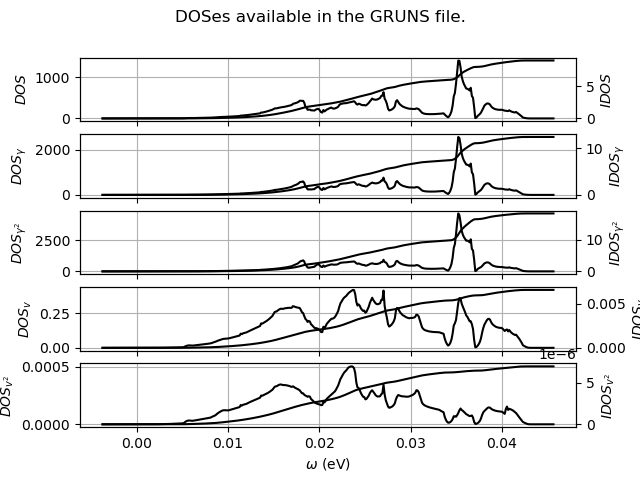
# Plot phonon DOSes computed by anaddb.
ncfile.plot_doses(title="DOSes available in the GRUNS file.")

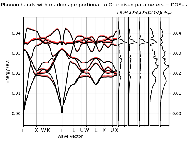
# Plot phonon bands with markers
# sphinx_gallery_thumbnail_number = 2
ncfile.plot_phbands_with_gruns(title="Phonon bands with markers proportional to Gruneisen parameters + DOSes")

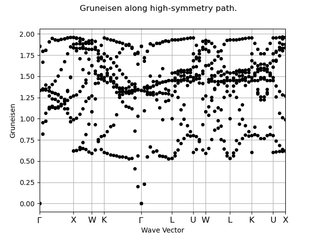
ncfile.plot_gruns_bs(title="Gruneisen along high-symmetry path.")

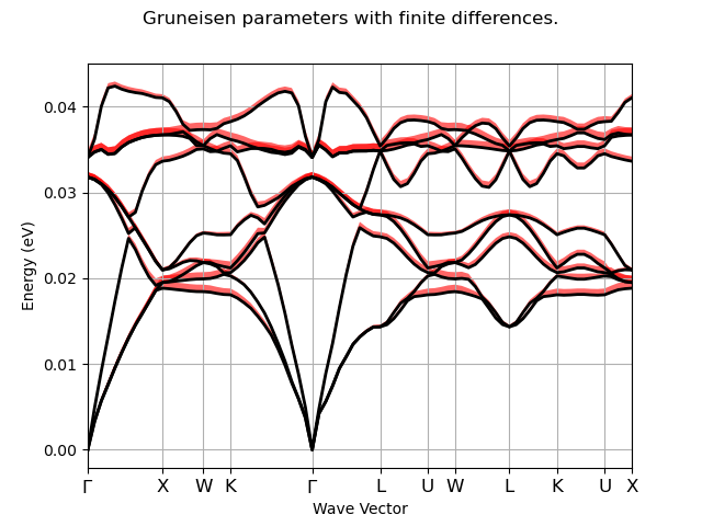
ncfile.plot_phbands_with_gruns(fill_with="gruns_fd",
                               title="Gruneisen parameters with finite differences.", with_doses=None)

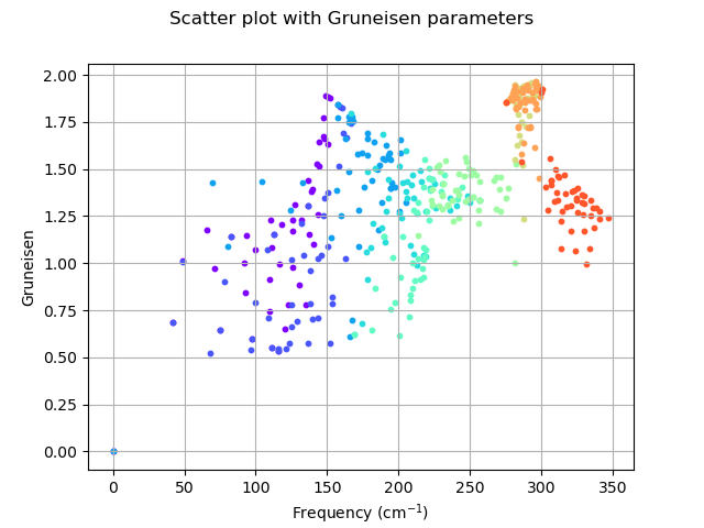
ncfile.plot_gruns_scatter(units='cm-1',title="Scatter plot with Gruneisen parameters")

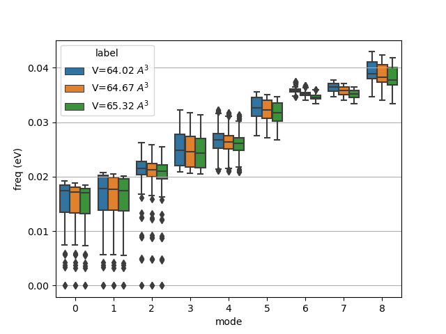
# Construct plotter object to analyze multiple phonon bands.
plotter = ncfile.get_plotter()
plotter.combiboxplot()

ncfile.close()