spin-polarized fatbands

This example shows how to plot the L-projected fatbands of Ni using the results stored in the FATBANDS.nc files produced with prtdos 3.

Open the file (alternatively one can use the shell and abiopen.py FILE -nb to open the file in a jupyter notebook This file has been produced on a k-path so it’s not suitable for DOS calculations.

import abipy.abilab as abilab
import abipy.data as abidata

fbnc_kpath = abilab.abiopen(abidata.ref_file("ni_kpath_FATBANDS.nc"))

NC files have contributions up to L = 4 (g channel) but here we are intererested in s,p,d terms only so we use the optional argument lmax

lmax = 2

# Energy limits in eV for plots. The pseudo contains semi-core states but
# we are not interested in this energy region. Fermi level set to zero.
elims = [-10, 2]

# Print file info (dimensions, variables ...)
# Note that prtdos = 3, so LM decomposition is not available.
print(fbnc_kpath)

# Plot the k-points belonging to the path.
#fbnc_kpath.ebands.kpoints.plot()

================================= File Info =================================
Name: ni_kpath_FATBANDS.nc
Directory: /home/runner/work/abipy/abipy/abipy/data/refs/ni_ebands
Size: 619.35 kB
Access Time: Tue Dec 24 15:33:49 2024
Modification Time: Tue Dec 24 15:29:30 2024
Change Time: Tue Dec 24 15:29:30 2024

================================= Structure =================================
Full Formula (Ni1)
Reduced Formula: Ni
abc   :   2.489016   2.489016   2.489016
angles:  60.000000  60.000000  60.000000
pbc   :       True       True       True
Sites (1)
  #  SP      a    b    c
---  ----  ---  ---  ---
  0  Ni      0    0    0

Abinit Spacegroup: spgid: 225, num_spatial_symmetries: 48, has_timerev: True, symmorphic: False

============================== Electronic Bands ==============================
================================= Structure =================================
Full Formula (Ni1)
Reduced Formula: Ni
abc   :   2.489016   2.489016   2.489016
angles:  60.000000  60.000000  60.000000
pbc   :       True       True       True
Sites (1)
  #  SP      a    b    c
---  ----  ---  ---  ---
  0  Ni      0    0    0

Abinit Spacegroup: spgid: 225, num_spatial_symmetries: 48, has_timerev: True, symmorphic: False

Number of electrons: 18.0, Fermi level: 11.296 (eV)
nsppol: 2, nkpt: 101, mband: 12, nspinor: 1, nspden: 2
smearing scheme: gaussian (occopt 7), tsmear_eV: 0.204, tsmear Kelvin: 2368.3

=============================== Fatbands Info ===============================
prtdos: 3, prtdosm: 1, mbesslang: 5, pawprtdos: 0, usepaw: 0
nsppol: 2, nkpt: 101, mband: 12

  Idx  Symbol    Reduced_Coords             Lmax    Ratsph [Bohr]  Has_Atom
-----  --------  -----------------------  ------  ---------------  ----------
    0  Ni        0.00000 0.00000 0.00000       4                2  Yes

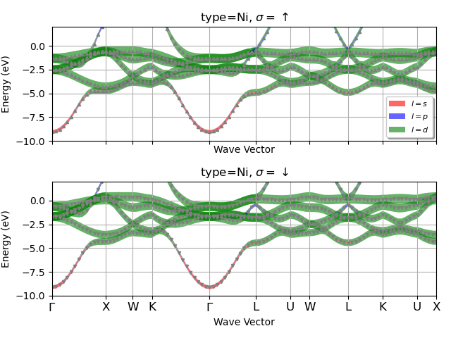
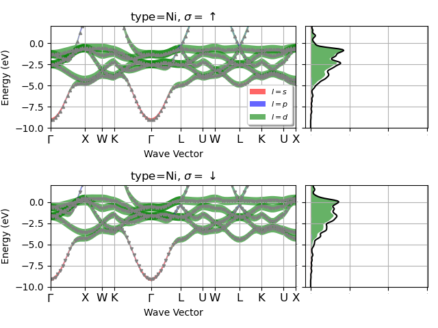
Plot the electronic fatbands grouped by atomic type.

fbnc_kpath.plot_fatbands_typeview(ylims=elims, lmax=lmax, tight_layout=True)

For the plotly version use:

fbnc_kpath.plotly_fatbands_typeview(ylims=elims, lmax=lmax)

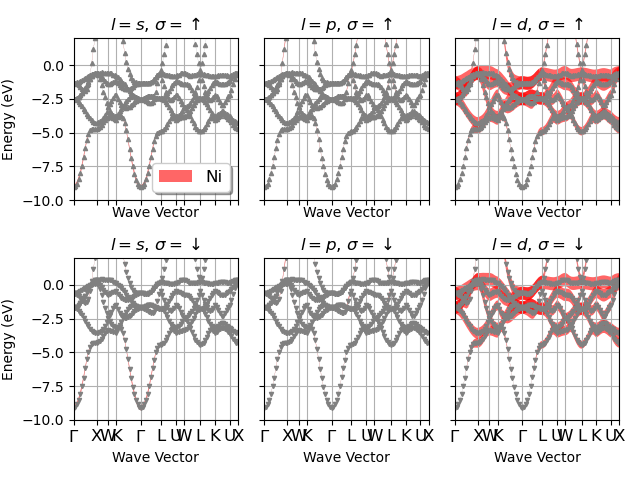
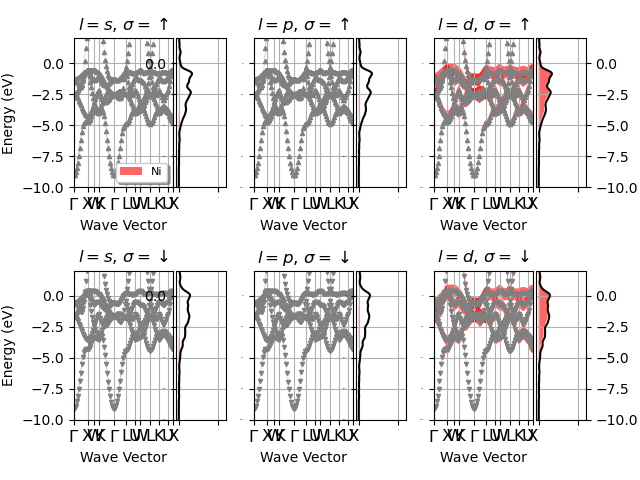
Plot the electronic fatbands grouped by L.

fbnc_kpath.plot_fatbands_lview(ylims=elims, lmax=lmax, tight_layout=True)

For the plotly version use:

fbnc_kpath.plotly_fatbands_lview(ylims=elims, lmax=lmax)

Now we read another FATBANDS file produced on 18x18x18 k-mesh

fbnc_kmesh = abilab.abiopen(abidata.ref_file("ni_666k_FATBANDS.nc"))

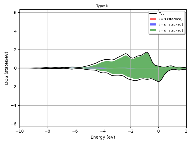
Plot the L-PJDOS grouped by atomic type.

fbnc_kmesh.plot_pjdos_typeview(xlims=elims, lmax=lmax, tight_layout=True)

For the plotly version use:

fbnc_kmesh.plotly_pjdos_typeview(xlims=elims, lmax=lmax)

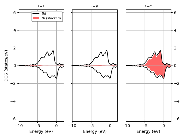
Plot the L-PJDOS grouped by L.

fbnc_kmesh.plot_pjdos_lview(xlims=elims, lmax=lmax, tight_layout=True)

For the plotly version use:

fbnc_kmesh.plotly_pjdos_lview(xlims=elims, lmax=lmax)

Now we use the two netcdf files to produce plots with fatbands + PJDOSEs. The data for the DOS is taken from pjdosfile.

fbnc_kpath.plot_fatbands_with_pjdos(pjdosfile=fbnc_kmesh,
                                    ylims=elims, lmax=lmax, view="type", tight_layout=True)

For the plotly version use:

fbnc_kpath.plotly_fatbands_with_pjdos(pjdosfile=fbnc_kmesh,
                                      ylims=elims, lmax=lmax, view="type")

fatbands + PJDOS grouped by L

fbnc_kpath.plot_fatbands_with_pjdos(pjdosfile=fbnc_kmesh,
                                    ylims=elims, lmax=lmax, view="lview", tight_layout=True)

For the plotly version use:

fbnc_kpath.plotly_fatbands_with_pjdos(pjdosfile=fbnc_kmesh,
                                      ylims=elims, lmax=lmax, view="lview")

Close files.

fbnc_kpath.close()
fbnc_kmesh.close()