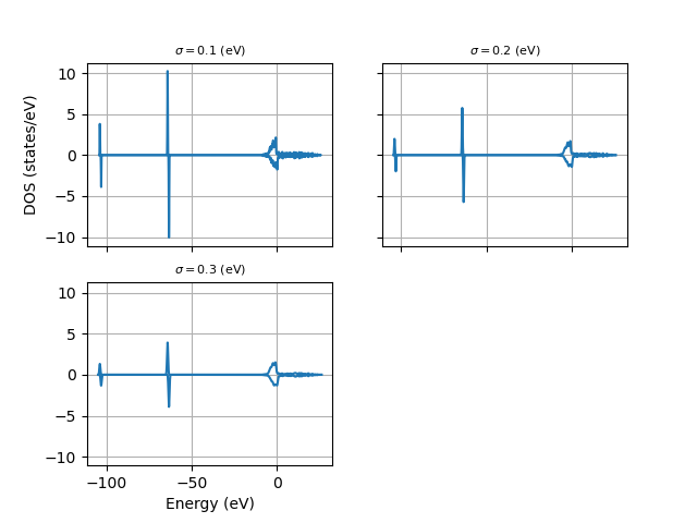
Multiple e-DOSes

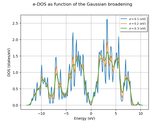
This example shows how to compute and plot multiple electron DOSes obtained with different values of the gaussian broadening.

• 
• 
• 
• 
• 
• 

import abipy.data as abidata

from abipy import abilab

# Open the wavefunction file computed with a homogeneous sampling of the BZ
# and extract the band structure on the k-mesh.
with abilab.abiopen(abidata.ref_file("si_scf_WFK.nc")) as gs_wfk:
    gs_bands = gs_wfk.ebands

# Compute the DOS with different values of the Gaussian smearing.
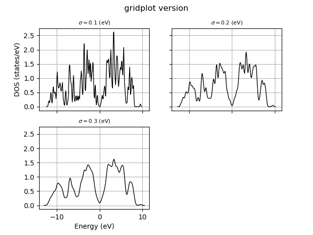
widths = [0.1, 0.2, 0.3]

edos_plotter = gs_bands.compare_gauss_edos(widths, step=0.1)

title = "e-DOS of Si for different Gaussian broadenings"

# Invoke ElectronDosPlotter methods to plot results.
edos_plotter.combiplot(title=title)

edos_plotter.gridplot(title=f"{title} (gridplot version)")

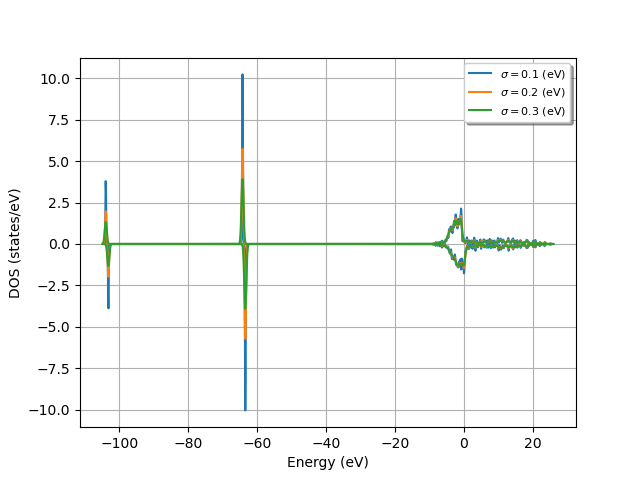
# Now we read the band structure of Nickel (spin-polarized)

with abilab.abiopen(abidata.ref_file("ni_666k_GSR.nc")) as gsr:
    ni_ebands_kmesh = gsr.ebands

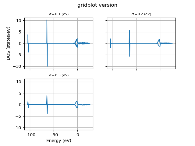
widths = [0.1, 0.2, 0.3]
edos_plotter = ni_ebands_kmesh.compare_gauss_edos(widths=widths, step=0.2)

title = "e-DOS of Ni for different Gaussian broadenings"

edos_plotter.combiplot(dos_mode="idos+dos", title=title)

edos_plotter.combiplot(dos_mode="dos", spin_mode="resolved",
                       title=f"{title} (spin-resolved)")

edos_plotter.gridplot(title=f"{title} (gridplot version)")

edos_plotter.gridplot(spin_mode="resolved",
                      title=f"{title} (gridplot version, spin-resolved)")