Optic results

This example shows how to plot the optical properties computed by optic within the independent-particle approximation, no local-field effects and no excitonic effects.

• 
• 
• 
• 

from abipy import abilab
import abipy.data as abidata

# Here we use one of the OPTIC.nc files shipped with abipy.
# Replace filename with the path to your OPTIC.nc file.
filename = abidata.ref_file("gaas_121212_OPTIC.nc")

ncfile = abilab.abiopen(filename)

# Optic files have a Structure and an ElectronBands object.
#ncfile.ebands.plot()

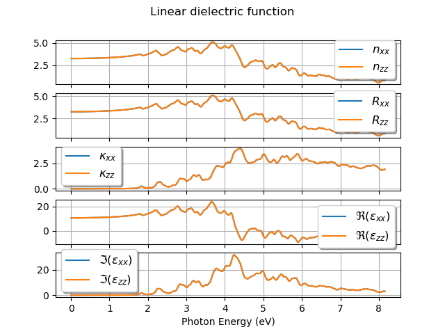
# To plot linear dielectric tensor and other optical
# properties for all tensor components available in the file:
ncfile.plot_linopt(title="Linear dielectric function")

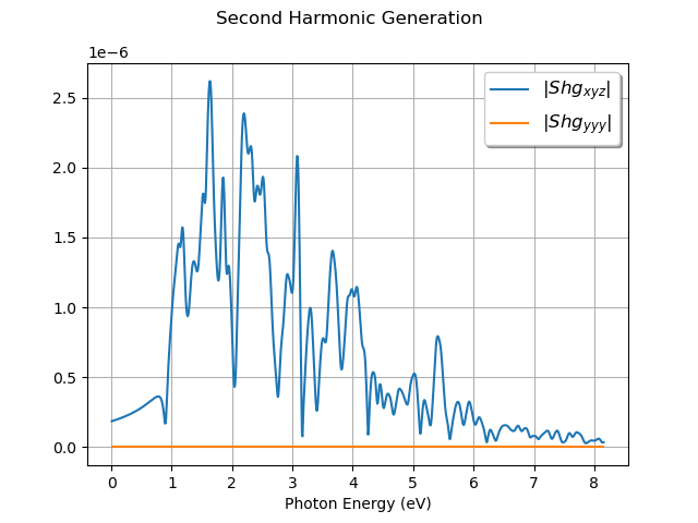
# To plot the second Harmonic tensor
ncfile.plot_shg(title="Second Harmonic Generation")

# Remember to close the file.
ncfile.close()

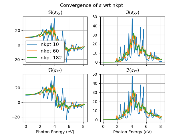
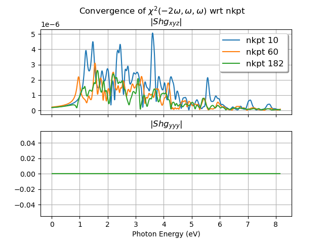
# Use OpticRobot to analyze multiple file e.g. convergence studies.
filenames = [
    abidata.ref_file("gaas_444_OPTIC.nc"),
    abidata.ref_file("gaas_888_OPTIC.nc"),
    abidata.ref_file("gaas_121212_OPTIC.nc"),
]

robot = abilab.OpticRobot.from_files(filenames)

# sphinx_gallery_thumbnail_number = 3
robot.plot_linopt_convergence(title=r"Convergence of $\epsilon$ wrt nkpt")

robot.plot_shg_convergence(title=r"Convergence of $\chi^2(-2\omega,\omega,\omega)$ wrt nkpt")

# Remember to close the file or use the `with` context manager.
robot.close()