Note
Go to the end to download the full example code.
Phonon convergence of ε∞, BECS, phonons and quadrupoles
This example shows how to use the DdbRobot to analyze the convergence of eps_inf, BECS, phonons and dynamical quadrupole with respect to the number of k-points.
import os

import abipy.data as abidata
Initialize the DdbRobot from a list of paths to DDB files Here we use DDB files shipped with the AbiPy package in data/refs/alas_eps_and_becs_vs_ngkpt Each DDB has been computed with a different k-mesh.
paths = ["AlAs_222k_DDB", "AlAs_444k_DDB", "AlAs_666k_DDB", "AlAs_888k_DDB"]
paths = [os.path.join(abidata.dirpath, "refs", "alas_eps_and_becs_vs_ngkpt", f) for f in paths]

from abipy.dfpt.ddb import DdbRobot

ddb_robot = DdbRobot.from_files(paths)
Call anaddb to get ε∞ for all the DDB files. Results and metadata are stored in the epsinf_data.df dataframe.
epsinf_data = ddb_robot.anacompare_epsinf()

print("ε∞ dataframe:\n", epsinf_data.df)

epsinf_data.plot_conv("nkpt", abs_conv=0.1)
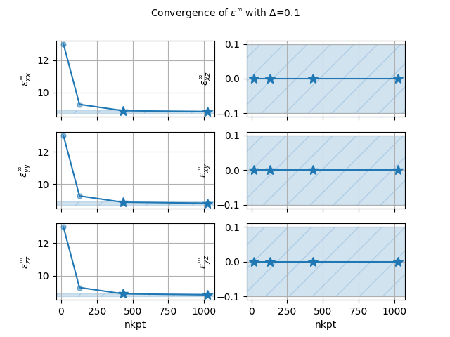
ε∞ dataframe:
           xx         yy         zz   yz   xz   xy  formula  chneut  nkpt
0  12.996449  12.996449  12.996449  0.0  0.0  0.0  Al1 As1       1    16
1   9.268431   9.268431   9.268431  0.0  0.0  0.0  Al1 As1       1   128
2   8.881665   8.881665   8.881665  0.0  0.0  0.0  Al1 As1       1   432
3   8.818122   8.818122   8.818122  0.0  0.0  0.0  Al1 As1       1  1024
Call anaddb to get BECs for all the DDB files. Results and metadata are stored in the becs_data.df dataframe.
becs_data = ddb_robot.anacompare_becs()
print("BECS dataframe:\n", becs_data.df)

becs_data.plot_conv("nkpt", abs_conv=0.1)
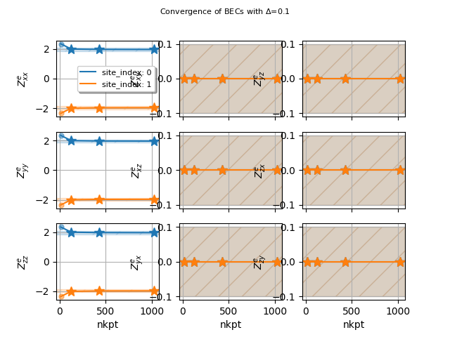
BECS dataframe:
   element  site_index         frac_coords wyckoff  ...   zy  formula  chneut  nkpt
0      Al           0     [0.0, 0.0, 0.0]      1a  ...  0.0  Al1 As1       1    16
2      Al           0     [0.0, 0.0, 0.0]      1a  ...  0.0  Al1 As1       1   128
6      Al           0     [0.0, 0.0, 0.0]      1a  ...  0.0  Al1 As1       1  1024
4      Al           0     [0.0, 0.0, 0.0]      1a  ...  0.0  Al1 As1       1   432
3      As           1  [0.25, 0.25, 0.25]      1d  ...  0.0  Al1 As1       1   128
1      As           1  [0.25, 0.25, 0.25]      1d  ...  0.0  Al1 As1       1    16
5      As           1  [0.25, 0.25, 0.25]      1d  ...  0.0  Al1 As1       1   432
7      As           1  [0.25, 0.25, 0.25]      1d  ...  0.0  Al1 As1       1  1024

[8 rows x 16 columns]
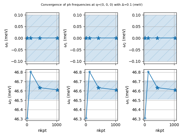
Call anaddb to get phonons at a single q-point for all the DDB files. Results and metadata are stored in the ph_data.ph_df dataframe.
ph_data = ddb_robot.get_phdata_at_qpoint(qpoint=(0, 0, 0))

print(ph_data.ph_df)
ph_data.plot_ph_conv("nkpt", abs_conv=0.1)  # meV units.
Calculation completed. Anaddb results available in: /tmp/tmph8l_nove
Calculation completed. Anaddb results available in: /tmp/tmp9ww8bfhl
Calculation completed. Anaddb results available in: /tmp/tmpj29e8071
Calculation completed. Anaddb results available in: /tmp/tmp2nn2ux4c
                                                    mode0  ...  spglib_lattice_type
../../data/refs/alas_eps_and_becs_vs_ngkpt/AlAs...    0.0  ...                cubic
../../data/refs/alas_eps_and_becs_vs_ngkpt/AlAs...    0.0  ...                cubic
../../data/refs/alas_eps_and_becs_vs_ngkpt/AlAs...    0.0  ...                cubic
../../data/refs/alas_eps_and_becs_vs_ngkpt/AlAs...    0.0  ...                cubic

[4 rows x 27 columns]
If the DDB contains dynamical quadrupoles, a similar dataframe with Q^* is automatically built and made available in ph_data.dyn_quad_df. A negative value of abs_conv is interpreted as relative convergence.
print(ph_data.dyn_quad_df)
ph_data.plot_dyn_quad_conv("nkpt", abs_conv=-0.02)
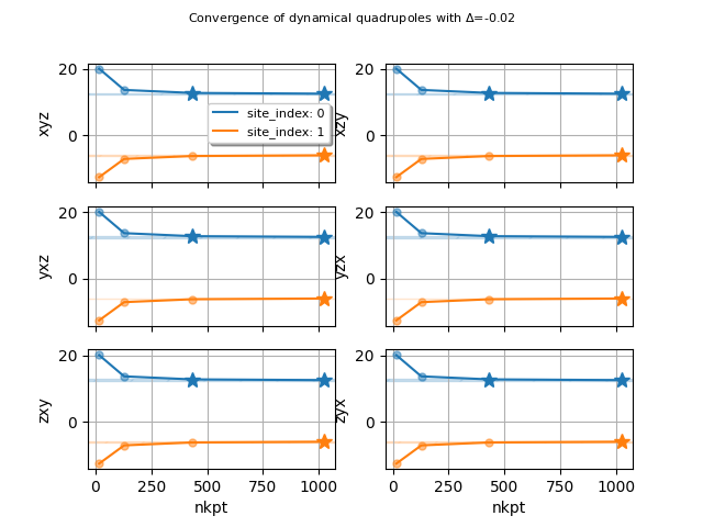
  element  site_index         frac_coords wyckoff  ...  occopt  ixc  nband  usepaw
0      Al           0     [0.0, 0.0, 0.0]      1a  ...       1    1      4       0
1      As           1  [0.25, 0.25, 0.25]      1d  ...       1    1      4       0
2      Al           0     [0.0, 0.0, 0.0]      1a  ...       1    1      4       0
3      As           1  [0.25, 0.25, 0.25]      1d  ...       1    1      4       0
4      Al           0     [0.0, 0.0, 0.0]      1a  ...       1    1      4       0
5      As           1  [0.25, 0.25, 0.25]      1d  ...       1    1      4       0
6      Al           0     [0.0, 0.0, 0.0]      1a  ...       1    1      4       0
7      As           1  [0.25, 0.25, 0.25]      1d  ...       1    1      4       0

[8 rows x 52 columns]
Total running time of the script: (0 minutes 9.615 seconds)