ElectronBandsPlotter

This example shows how to plot several band structures on a grid

We use two GSR files:

si_scf_GSR.n: energies on a homogeneous sampling of the BZ (can be used to compute DOS) si_nscf_GSR.nc: energies on a k-path in the BZ (used to plot the band dispersion)

from abipy.abilab import ElectronBandsPlotter
from abipy.data import ref_file

# To plot a grid with two band structures:
plotter = ElectronBandsPlotter()
plotter.add_ebands("BZ sampling", ref_file("si_scf_GSR.nc"))
plotter.add_ebands("k-path", ref_file("si_nscf_GSR.nc"))

# Get pandas dataframe
frame = plotter.get_ebands_frame()
print(frame)

Out:

             nsppol  nspinor  ...                      dirgap_kstart                        dirgap_kend
BZ sampling       1        1  ...           [+0.000, +0.000, +0.000]           [+0.000, +0.000, +0.000]
k-path            1        1  ...  [+0.000, +0.000, +0.000] $\Gamma$  [+0.000, +0.000, +0.000] $\Gamma$

[2 rows x 31 columns]

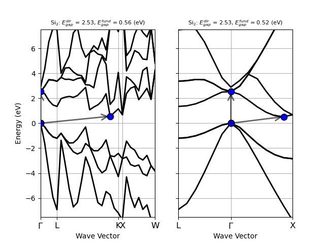
To create a grid plot use:

plotter.gridplot(with_gaps=True)

Out:

<Figure size 640x480 with 2 Axes>

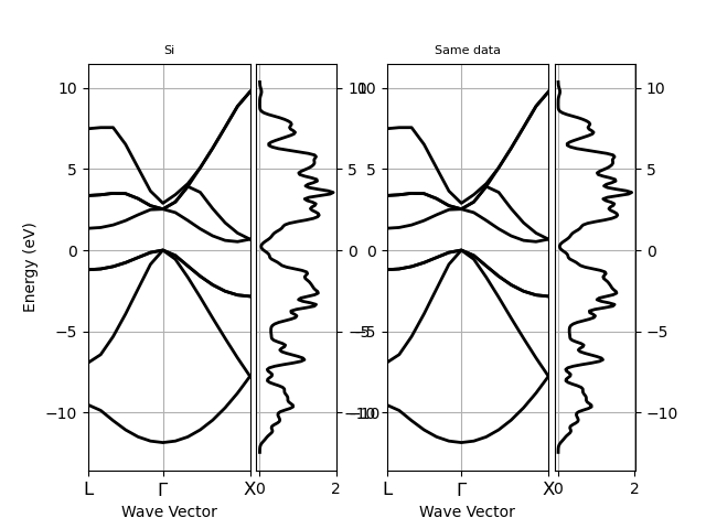
To plot a grid with band structures + DOS, use the optional argument edos_objects The first subplot gets the band dispersion from eb_objects[0] and the DOS from edos_objects[0] edos_kwargs is an optional dictionary passed to get_dos to compute the DOS.

eb_objects = 2 * [ref_file("si_nscf_GSR.nc")]
edos_objects = 2 * [ref_file("si_scf_GSR.nc")]

plotter = ElectronBandsPlotter()
plotter.add_ebands("Si", ref_file("si_nscf_GSR.nc"), edos=ref_file("si_scf_GSR.nc"))
plotter.add_ebands("Same data", ref_file("si_nscf_GSR.nc"), edos=ref_file("si_scf_GSR.nc"))
# sphinx_gallery_thumbnail_number = 2
plotter.gridplot()

Out:

<Figure size 640x480 with 4 Axes>