Visualization of GWR results

This example shows how to visualize the results produced by the GWR code.

from abipy import abilab
import abipy.data as abidata

Open the GWR.nc file Here we use one of the GSR files shipped with abipy. Replace filename with the path to your GSR file or your WFK file.

from abipy.electrons.gwr import GwrFile
gwr = GwrFile(abidata.ref_file("t01o_DS3_GWR.nc"))
print(gwr)

kpoint = 0
include_bands = "gap"

================================= File Info =================================
Name: t01o_DS3_GWR.nc
Directory: /home/runner/work/abipy/abipy/abipy/data/refs/gwr
Size: 124.86 kB
Access Time: Thu Jan 23 22:36:34 2025
Modification Time: Thu Jan 23 22:30:41 2025
Change Time: Thu Jan 23 22:30:41 2025

================================= Structure =================================
Full Formula (Si2)
Reduced Formula: Si
abc   :   3.839136   3.839136   3.839136
angles:  60.000000  60.000000  60.000000
pbc   :       True       True       True
Sites (2)
  #  SP       a     b     c
---  ----  ----  ----  ----
  0  Si    0     0     0
  1  Si    0.25  0.25  0.25

Abinit Spacegroup: spgid: 227, num_spatial_symmetries: 48, has_timerev: True, symmorphic: True

============================= KS Electron Bands =============================
Number of electrons: 8.0, Fermi level: -0.451 (eV)
nsppol: 1, nkpt: 3, mband: 40, nspinor: 1, nspden: 1
smearing scheme: none (occopt 1), tsmear_eV: 0.272, tsmear Kelvin: 3157.7
Direct gap:
    Energy: 2.454 (eV)
    Initial state: spin: 0, kpt: [+0.000, +0.000, +0.000], weight: 0.125, band: 3, eig: -0.451, occ: 2.000
    Final state:   spin: 0, kpt: [+0.000, +0.000, +0.000], weight: 0.125, band: 4, eig: 2.003, occ: 0.000
Fundamental gap:
    Energy: 0.903 (eV)
    Initial state: spin: 0, kpt: [+0.000, +0.000, +0.000], weight: 0.125, band: 3, eig: -0.451, occ: 2.000
    Final state:   spin: 0, kpt: [+0.500, +0.500, +0.000], weight: 0.375, band: 4, eig: 0.451, occ: 0.000
Bandwidth: 11.636 (eV)
Valence maximum located at kpt index 0:
    spin: 0, kpt: [+0.000, +0.000, +0.000], weight: 0.125, band: 3, eig: -0.451, occ: 2.000
Conduction minimum located at kpt index 2:
    spin: 0, kpt: [+0.500, +0.500, +0.000], weight: 0.375, band: 4, eig: 0.451, occ: 0.000

TIP: Use `--verbose` to print k-point coordinates with more digits

=============================== GWR parameters ===============================
gwr_task: G0W0
Number of k-points in Sigma_{nk}: 2
Number of bands included in e-e self-energy sum: 40
ecuteps: 4.0
ecutsigx: 4.0
ecut: 4.0
gwr_boxcutmin: 1.1

============================ QP direct gaps in eV ============================
            kpoint     kname  ks_dirgaps  qpz0_dirgaps  spin
0  [0.0, 0.0, 0.0]  $\Gamma$    2.454214      3.274460     0
1  [0.5, 0.0, 0.0]         L    3.496978      4.281203     0

Plot Sigma_nk(iw) along the imaginary axis for given k-point.

gwr.plot_sigma_imag_axis(kpoint=kpoint, include_bands=include_bands)

Plot Sigma_nk(iw) along the real axis for given k-point.

gwr.plot_sigma_real_axis(kpoint=kpoint)

Plot the spectral function A(w) along the real axis.

gwr.plot_spectral_functions()

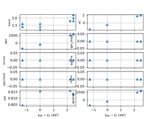
Plot qp-data versus KS energy

gwr.plot_qps_vs_e0()