Dielectric function with LFE

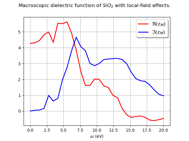
This examples shows how to plot the macroscopic dielectric function computed in the GW code (optdriver 3)

• 
• 
• 

================================= File Info =================================
Name: sio2_SCR.nc
Directory: /home/runner/work/abipy/abipy/abipy/data/refs/sio2_screening
Size: 426.16 kB
Access Time: Tue Dec 24 15:33:28 2024
Modification Time: Tue Dec 24 15:29:30 2024
Change Time: Tue Dec 24 15:29:30 2024

================================= Structure =================================
Full Formula (Si3 O6)
Reduced Formula: SiO2
abc   :   4.913040   4.913040   5.404630
angles:  90.000000  90.000000 120.000000
pbc   :       True       True       True
Sites (9)
  #  SP         a       b          c
---  ----  ------  ------  ---------
  0  Si     0.465   0       0
  1  Si     0       0.465   0.666667
  2  Si    -0.465  -0.465   0.333333
  3  O      0.415   0.272   0.12
  4  O     -0.143  -0.415   0.453333
  5  O     -0.272   0.143   0.786667
  6  O      0.143  -0.272  -0.12
  7  O      0.272   0.415   0.546667
  8  O     -0.415  -0.143   0.213333

Abinit Spacegroup: spgid: 0, num_spatial_symmetries: 6, has_timerev: True, symmorphic: True

====================== K-points for screening function ======================
0) [+0.000, +0.000, +0.000]
1) [+0.250, +0.000, +0.000]
2) [+0.500, +0.000, +0.000]
3) [+0.250, +0.250, +0.000]
4) [+0.000, +0.000, +0.333]
5) [+0.250, +0.000, +0.333]
6) [+0.500, +0.000, +0.333]
7) [-0.250, +0.000, +0.333]
8) [+0.250, +0.250, +0.333]

Number of G-vectors in screening matrices: 9
Number of frequencies: 35 (real: 30, imaginary: 5)
Setting Fermi energy to zero since `fermie_energy` is not initialized in Abinit v8.2

import abipy.data as abidata
from abipy.abilab import abiopen

with abiopen(abidata.ref_file("sio2_SCR.nc")) as ncfile:
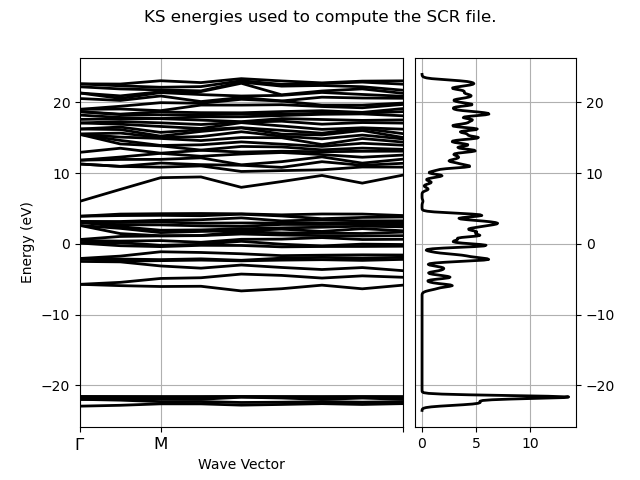
    # The SCR file contains a structure and electron bands in the IBZ.
    # We can thus use the ebands object to plot bands + DOS.
    print(ncfile)

    edos = ncfile.ebands.get_edos()
    ncfile.ebands.plot_with_edos(edos, title="KS energies used to compute the SCR file.")

    # sphinx_gallery_thumbnail_number = 2
    ncfile.plot_emacro(title="Macroscopic dielectric function of $SiO_2$ with local-field effects.")

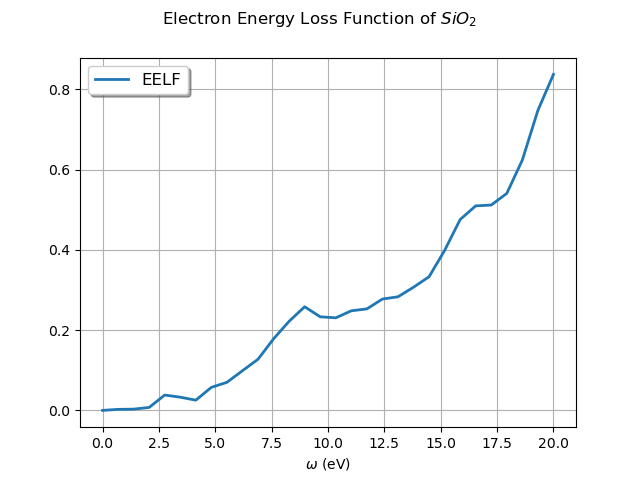
    ncfile.plot_eelf(title="Electron Energy Loss Function of $SiO_2$")