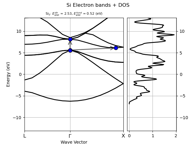
Bands + DOS

This example shows how to compute the DOS and plot a band structure with DOS using two GSR files.

from abipy.abilab import abiopen
import abipy.data as abidata

# Open the file with energies computed on a k-path in the BZ
# and extract the band structure object.
with abiopen(abidata.ref_file("si_nscf_GSR.nc")) as nscf_file:
    nscf_ebands = nscf_file.ebands

# Open the file with energies computed with a homogeneous sampling of the BZ
# and extract the band structure object.
with abiopen(abidata.ref_file("si_scf_GSR.nc")) as gs_file:
    gs_ebands = gs_file.ebands

Compute the DOS with the Gaussian method (use default values for the broadening and the step of the linear mesh.

edos = gs_ebands.get_edos()

To plot bands and DOS with matplotlib use:

nscf_ebands.plot_with_edos(edos, with_gaps=True, title="Si Electron bands + DOS")

For the plotly version use:

nscf_ebands.plotly_with_edos(edos, with_gaps=True, title="Si Electron bands + DOS")