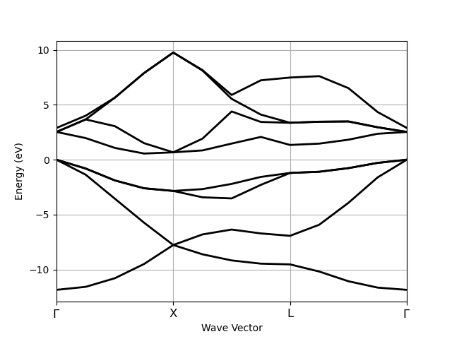
K-path from IBZ

This example shows how to extract energies along a k-path from a calculation done with a (relatively dense) IBZ sampling.

Out:

K-mesh with divisions: [8, 8, 8], shifts: [0.0, 0.0, 0.0]
kptopt: 1 (Use space group symmetries and TR symmetry)
Number of points in the IBZ: 29
     0) [+0.000, +0.000, +0.000],  weight=0.002
     1) [+0.125, +0.000, +0.000],  weight=0.016
     2) [+0.250, +0.000, +0.000],  weight=0.016
     3) [+0.375, +0.000, +0.000],  weight=0.016
     4) [+0.500, +0.000, +0.000],  weight=0.008
     5) [+0.125, +0.125, +0.000],  weight=0.012
     6) [+0.250, +0.125, +0.000],  weight=0.047
     7) [+0.375, +0.125, +0.000],  weight=0.047
     8) [+0.500, +0.125, +0.000],  weight=0.047
     9) [-0.375, +0.125, +0.000],  weight=0.047
    10) [-0.250, +0.125, +0.000],  weight=0.047
    ... (More than 10 k-points)
================================= Structure =================================
Full Formula (Si2)
Reduced Formula: Si
abc   :   3.866975   3.866975   3.866975
angles:  60.000000  60.000000  60.000000
Sites (2)
  #  SP       a     b     c  cartesian_forces
---  ----  ----  ----  ----  -----------------------------------------------------------
  0  Si    0     0     0     [-5.89948306e-27 -1.93366149e-27  2.91016904e-27] eV ang^-1
  1  Si    0.25  0.25  0.25  [ 5.89948306e-27  1.93366149e-27 -2.91016904e-27] eV ang^-1

Abinit Spacegroup: spgid: 227, num_spatial_symmetries: 48, has_timerev: True, symmorphic: True

Number of electrons: 8.0, Fermi level: 5.598 (eV)
nsppol: 1, nkpt: 13, mband: 8, nspinor: 1, nspden: 1
smearing scheme: none (occopt 1), tsmear_eV: 0.272
Direct gap:
    Energy: 2.532 (eV)
    Initial state: spin: 0, kpt: [+0.000, +0.000, +0.000], weight: 0.000, band: 3, eig: 5.598, occ: 2.000
    Final state:   spin: 0, kpt: [+0.000, +0.000, +0.000], weight: 0.000, band: 4, eig: 8.130, occ: 0.000
Fundamental gap:
    Energy: 0.562 (eV)
    Initial state: spin: 0, kpt: [+0.000, +0.000, +0.000], weight: 0.000, band: 3, eig: 5.598, occ: 2.000
    Final state:   spin: 0, kpt: [+0.375, +0.000, +0.375], weight: 0.000, band: 4, eig: 6.161, occ: 0.000
Bandwidth: 11.856 (eV)
Valence maximum located at:
    spin: 0, kpt: [+0.000, +0.000, +0.000], weight: 0.000, band: 3, eig: 5.598, occ: 2.000
Conduction minimum located at:
    spin: 0, kpt: [+0.375, +0.000, +0.375], weight: 0.000, band: 4, eig: 6.161, occ: 0.000

TIP: Call set_fermie_to_vbm() to set the Fermi level to the VBM if this is a non-magnetic semiconductor


<Figure size 640x480 with 1 Axes>

from abipy.abilab import abiopen
import abipy.data as abidata

# Open the file with energies computed with a homogeneous sampling of the BZ
# and extract the band structure object.
with abiopen(abidata.ref_file("si_scf_GSR.nc")) as gs_file:
    ebands_ibz = gs_file.ebands

# This is a GS calculation done with a 8x8x8 k-mesh.
print(ebands_ibz.kpoints)

# Build new ebands with energies along G-X-L-G path.
# Smooth bands require dense meshes.
r = ebands_ibz.with_points_along_path(knames=["G", "X", "L", "G"])

print(r.ebands)
r.ebands.plot()