GW Convergence

This example shows how to use the SigresRobot to visualize the convergence of the QP results stored in the SIGRES.nc files produced by the GW code (sigma run).

• 
• 
• 

Out:

<Figure size 640x480 with 1 Axes>

from abipy.abilab import SigresRobot
import abipy.data as abidata

# List of SIGRES files computed with different values of nband.
filenames = [
    "si_g0w0ppm_nband10_SIGRES.nc",
    "si_g0w0ppm_nband20_SIGRES.nc",
    "si_g0w0ppm_nband30_SIGRES.nc",
]

filepaths = [abidata.ref_file(fname) for fname in filenames]

# Build robot from list of file paths
robot = SigresRobot.from_files(filepaths)
#robot.remap_labels(lambda sigres: sigres.params["sigma_nband"])

# Plot the convergence of the QP gaps.
robot.plot_qpgaps_convergence(sortby="sigma_nband", title="QP gaps vs sigma_nband")

# Plot the convergence of the QP energies.
robot.plot_qpdata_conv_skb(spin=0, kpoint=[0, 0, 0], band=3, sortby="sigma_nband")

# sphinx_gallery_thumbnail_number = 3
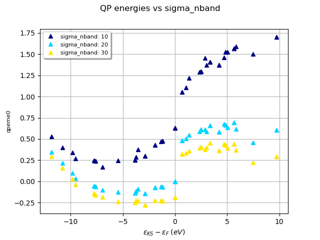
robot.plot_qpfield_vs_e0("qpeme0", sortby="sigma_nband", title="QP energies vs sigma_nband")