Joint Density of States

This example shows how plot the different contributions to the electronic joint density of states of Silicon

• 
• 
• 

import abipy.data as abidata
from abipy.abilab import abiopen

# Extract the bands computed with the SCF cycle on a Monkhorst-Pack mesh.
with abiopen(abidata.ref_file("si_scf_WFK.nc")) as wfk_file:
    ebands = wfk_file.ebands

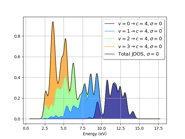
# Select the valence and conduction bands to include in the JDOS
# Here we include valence bands from 0 to 3 and the first conduction band (4).
vrange = range(0, 4)
crange = range(4, 5)

# Plot joint-DOS.
ebands.plot_ejdosvc(vrange, crange)

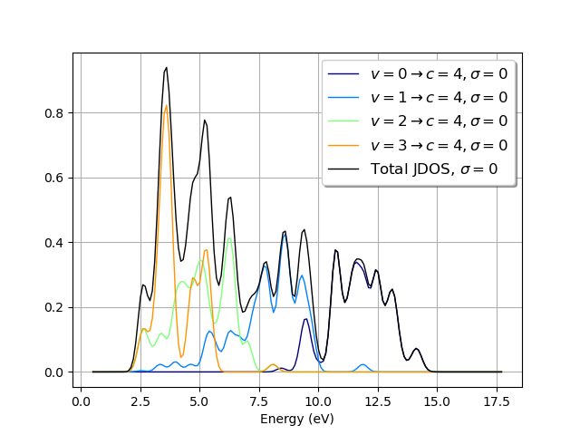
# Plot decomposition of joint-DOS in terms of v --> c transitions
ebands.plot_ejdosvc(vrange, crange, cumulative=False)

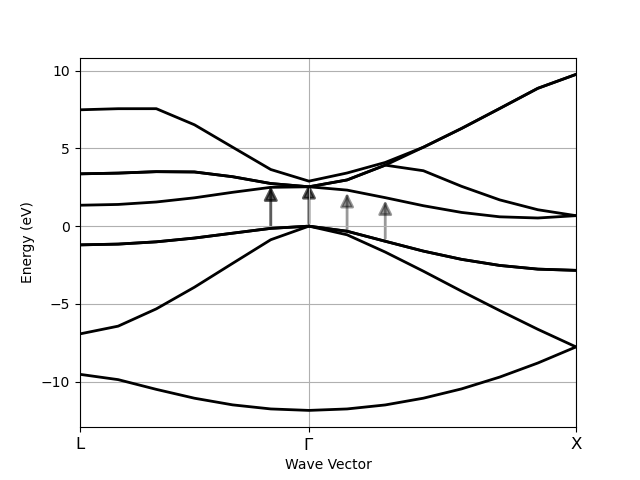
# Show optical (vertical) transitions of energy 2.8 eV
with abiopen(abidata.ref_file("si_nscf_GSR.nc")) as gsr_file:
    gsr_file.ebands.plot_transitions(2.8)